Numerical solution of ordinary differential equations: Higher order Runge-Kutta methods

As always, we start by importing some important Python modules.

Show code cell source Hide code cell source

import numpy as np
from numpy import pi
from numpy.linalg import solve, norm    
import matplotlib.pyplot as plt
    

# Use a funny plotting style
# plt.xkcd()
newparams = {'figure.figsize': (6.0, 6.0), 'axes.grid': True,
             'lines.markersize': 8, 'lines.linewidth': 2,
             'font.size': 14}
plt.rcParams.update(newparams)

Runge-Kutta Methods

In the previous lectures we introduced Euler’s method and Heun’s method as particular instances of the One Step Methods, and we presented the general error theory for one step method.

In this note we will consider one step methods which go under the name Runge-Kutta methods (RKM). We will see that Euler’s method and Heun’s method are instance of RKMs. But before we start, we will derive yet another one-step method, known as explicit midpoint rule or improved explicit Euler method.

As for Heun’s method, we start from the IVP \(y' = f(t, y)\), integrate over \([t_k, t_{k+1}]\) and apply the midpoint rule:

\[ y(t_{k+1}) - y(t_k) = \int_{t_k}^{t_{k+1}} f(t, y(t)){\,\mathrm{d}t} \]

\[ \approx \tau_k f(t_k + \tfrac{1}{2}\tau_k, y(t_k + \tfrac{1}{2}\tau_k)) \]

Since we cannot determine the value \(y(t_k + \tfrac{1}{2}\tau_k)\) from this system, we borrow an idea from derivation of Heun’s method and approximate it using a half explicit Euler step

\[ y(t_k + \tfrac{1}{2}\tau_k) \approx y(t_k + \tfrac{1}{2}\tau_k f(t_k, y(t_k)), \]

leading to the following one-step methods: Given \(y_k, \tau_k\) and \(f\), compute

(14)\[ y_{k+1} := y_k + \tau_k f(t_k + \tfrac{1}{2}\tau_k, y_k + \tfrac{1}{2}\tau_k f(t_k, y_k)). \]

The nested function expression can again be rewritten using 2 stage derivatives, which leads to the following form of the explicit midpoint rule or improved explicit Euler method:

\[ k_{1} := f(t_k, y_k) \]

\[ k_{2} := f(t_k + \tfrac{\tau_k}{2}, y_k + \tfrac{\tau_k}{2} k_1) \]

\[ y_{k+1} := y_k + \tau_k k_2 \]

Exercise 19 (Analyzing the improved explicit Euler method)

a) Find the increment function \(\Phi\) for the improved explicit Euler method.

b) Assuming the right-hand side \(f\) of a given IVP satisfies a Lipschitz condition \(\| f(t, y) - f(t, z)\| \leqslant M \| y-z\| \) with a constant \(L_f\) independent of \(t\), show that the incremement function \(\Phi\) of the improved Euler method does also satisfies a Lipschitz condition for some constant \(L_{\Phi}\).

Hint. Get some inspiration from the corresponding result for Heun’s method derived in ErrorAnalysisNuMeODE notes.

c) Show the improved explicit Euler method is consistent of order \(2\) if the right-hand side \(f\) of a given IVP is in \(C^2\).

Hint. Get some inspiration from the corresponding result for Heun’s method derived in ErrorAnalysisNuMeODE notes.

Solution to Exercise 19 (Analyzing the improved explicit Euler method)

a)

\[ \Phi(t_k, y_{k}, \tau_{k}) = f\left(t_{k} + \frac{\tau}{2}, y_k + \frac{\tau}{2}f(t_k,y_k)\right). \]

b) Using the increment function above, the Lipschitz condition for \(f\), the triangle inequality and then the Lipschitz condition for \(f\) again we get the following:

\[\begin{align*} |\Phi(t,y)-\Phi(t,z)| &= |f\left(t + \frac{\tau}{2}, y + \frac{\tau}{2}f(t,y)\right) - f\left(t + \frac{\tau}{2}, z + \frac{\tau}{2}f(t,z)\right)| \\ &\leq M| y + \frac{\tau}{2}f(t,y) - z - \frac{\tau}{2}f(t,z) | \\ &\leq M| y - z | + M\frac{\tau}{2} | f(t,y) - f(t,z) | \\ &\leq M| y - z | + M^2\frac{\tau}{2} | y-z | \\ & = (M+\frac{\tau}{2}M^2)|y-z|. \end{align*}\]

Assuming that the step size \(\tau\) is bounded upward by some \(\tau_0\), we can conclude that

\[ |\Phi(t,y)-\Phi(t,z)| \leq L_{\Phi}|y-z|, \qquad L_{\Phi}=M+\frac{\tau_0}{2}M^2. \]

c) As before, we have the following for the exact solution:

\[ y(t_0+\tau) = y_0 + \tau f + \frac{\tau^2}{2}(f_t + f_y f) + \frac{\tau^3}{6}(f_{tt}+2f_{ty}f+f_{yy}ff + f_yf_xf + f_yf_t+ (f_y)^2f ) + \dotsm, \]

where \(f\) and all its derivatives are evaluated in \((t_0,y_0)\).

For the numerical solution we get

\[\begin{align*} k_1 &= f(t_0,y_0) = f, \\ k_2 &= f(t_0+\frac{\tau}{2}, y_0+\frac{\tau}{2} k_1) \\ & = f + \frac{\tau}{2} f_t + f_y\frac{\tau}{2} k_1 + \frac{1}{8}f_{tt}\tau^2 + f_{ty}\frac{\tau^2}{4} k_1 + \frac{1}{8}f_{yy}\tau^2 k_1^2 + \dotsm \\ &= f + \frac{\tau}{2}(f_t + f_yf) + \frac{\tau^2}{8}(f_{tt} + 2f_{ty}f + f_{yy}f^2) + \dotsm \\ y_1 &= \tau k_2 \end{align*}\]

and the local truncation error will be

\[ \eta(t_0, \tau) = y(t_0+\tau)-y_1 = \frac{\tau^3}{24}(-f_{tt}-2f_{ty}f-f_{yy}f^2 + 4f_yf_t + 4(f_y)^2f) + \dotsm \]

Recall that the explicit Euler method is defined by

(15)\[\begin{align} k_{1} &:= f(t_k, y_k) \\ y_{k+1} &:= y_k + \tau_k k_1 \end{align}\]

And Heun’s method or explicit trapezoidal rule is similar to the improved explicit Euler method given by

(16)\[\begin{align} k_{1} &:= f(t_k, y_k) \\ k_{2} &:= f(t_k + \tau_k, y_k + \tau_k k_1) \\ y_{k+1} &:= y_k + \tau_k ( \tfrac{1}{2} k_1 + \tfrac{1}{2} k_2 ) \end{align}\]

Note that for all schemes so far, we are able to successively compute the stage derivatives, starting from \(k_1 = f(t_k, y_{k})\).

This is not the case for the last one-step method we encountered so far, namely the implicit trapezoidal rule or Crank-Nicolson method:

\[ y_{k+1} := y_k + \tau_k (\tfrac{1}{2} \underbrace{f(t_k, y_k)}_{:=k_1} + \tfrac{1}{2} \underbrace{f(t_k+\tau_k, y_{k+1}))}_{:= k_2} \]

Using stage derivatives, we obtain this time

(17)\[\begin{align} k_{1} := f(t_k, y_k) \\ k_{2} := f(t_k + \tau_k, y_{k} + \tau (\tfrac{1}{2}k_1 + \tfrac{1}{2} k_2)) \\ y_{k+1} := y_k + \tau_k ( \dfrac{1}{2} k_1 + \dfrac{1}{2} k_2 ) \end{align}\]

The previous examples and the wish for constructing higher (\(> 2\)) one-step methods leads to following definition

Definition 7

Given \(b_j\), \(c_j\), and \(a_{jl}\) for \(j,l = 1,\ldots s\), a Runge-Kutta method is defined by the recipe

(18)\[\begin{align} k_{j} &:= f(t_k + c_j \tau, y_i + \tau_k \sum_{l=1}^{s} {a}_{jl} k_l) \quad j = 1,\ldots s, \\ y_{k+1} &:= y_{k} + \tau_k \sum_{j=1}^s b_j k_j \end{align}\]

Runge-Kutta schemes are often specified in the form of a Butcher table:

\[\begin{split} \begin{array}{c|ccc} c_1 & a_{11} & \cdots & a_{1s} \\ \vdots & \vdots & & \vdots \\ c_s & a_{s1} & \cdots & a_{ss} \\ \hline & b_1 & \cdots & b_s \end{array} \end{split}\]

If \(a_{ij} = 0\) for \(j \geqslant i\) the Runge-Kutta method is called explicit as the stages \(k_i\) are defined explicitly and can be computed successively:

\[ k_1 := f(t_k + c_1 \tau_k, y_k) \]

\[ k_2 := f(t_k + c_2 \tau_k, y_k + \tau_k a_{21} k_1) \]

\[ k_3 := f(t_k + c_3 \tau_k, y_k + \tau_k a_{31} k_1 + \tau a_{32} k_2) \]

\[ \vdots \]

\[ k_j := f(t_k + c_j \tau_k, y_k + \tau_k \sum_{l=1}^{j-1} a_{jl} k_l) \]

\[ \vdots \]

\[ k_s := f(t_k + c_s \tau_k, y_k + \tau_k \sum_{l=1}^{s-1} a_{sl} k_l) \]

\[ y_{k+1} := y_{k} + \tau \sum_{j=1}^s b_j k_j \]

Exercise 20 (Butcher tables for some well-known Runge-Kutta methods)

Write down the Butcher table for the

1. explicit Euler

2. Heun’s method (explicit trapezoidal rule)

3. Crank-Nicolson (implicit trapezoidal rule)

4. improved explicit Euler method (explicit midpoint rule)

and go to “www.menti.com” and take the quiz.

\[\begin{split} \boldsymbol{\mathrm{A})} \quad \begin{array}{c|c c} 0 & 0 & 0 \\ \tfrac{1}{2} & \tfrac{1}{2} & 0 \\ \hline & 0 & 1 \end{array} \qquad \boldsymbol{\mathrm{B})} \quad \begin{array}{c|c} 0 & 0 \\ \hline & 1 \end{array} \qquad \boldsymbol{\mathrm{C})} \quad \begin{array}{c|cc} 0 & 0 & 0 \\ 1 & 1 & 0 \\ \hline & \frac{1}{2} & \frac{1}{2} \end{array} \qquad \boldsymbol{\mathrm{D})} \quad \begin{array}{c|cc} 0 & 0 & 0 \\ 1 & \dfrac{1}{2} & \dfrac{1}{2} \\ \hline & \frac{1}{2} & \frac{1}{2} \end{array} \end{split}\]

Solution to Exercise 20 (Butcher tables for some well-known Runge-Kutta methods)

The correct pairing is

1. explicit Euler: \(\textbf{B)}\)

2. Heun’s method (explicit trapezoidal rule): \(\textbf{C)}\)

3. Crank-Nicolson (implicit trapezoidal rule): \(\textbf{D)}\)

4. improved explicit Euler method (explicit midpoint rule): \(\textbf{A)}\)

We show a verbose solution for explicit Euler, improved explicit Euler and Crank-Nicolson.

Explicit Euler method: Since we have only one stage derivative, this is an example of a 1-stage Runge-Kutta method (s=1). Looking at the definition of the stage and the final step, we see that

\[ k_{1} := f(t_k, y_k) = f(t_k + \underbrace{0}_{c_1} \cdot \tau_k, y_k + \tau_k \underbrace{0}_{a_{11}} \cdot k_1) \Rightarrow c_1 = a_{11} = 0 \]

\[ y_{k+1} := y_k + \tau_k k_1 = y_k + \tau_k \underbrace{1}_{b_1}\cdot k_1 \Rightarrow b_1 = 1 \]

Thus, the Butcher table is

\[\begin{split} \boldsymbol{\mathrm{B})} \quad \begin{array}{c|c} 0 & 0 \\ \hline & 1 \end{array} \end{split}\]

Improved explicit Euler method: Since we have to stage derivatives, this is an example of a 2-stage Runge-Kutta method (s=2). Looking at the definition of the stages and the final step, we see that

\[ k_{1} := f(t_k, y_k) = f(t_k + \underbrace{0}_{c_1} \cdot \tau_k, y_k + \tau_k \underbrace{0}_{a_{11}} \cdot k_1 + \tau_k \underbrace{0}_{a_{21}} \cdot k_2) \Rightarrow c_1 = a_{11} = a_{21} = 0 \]

\[ k_{2} := f(t_k + \tfrac{\tau_k}{2}, y_k + \tfrac{\tau_k}{2} k_1) \]

\[ \phantom{:}= f(t_k + \underbrace{\tfrac{1}{2}}_{c_2}\tau_k, y_k + \tau_k\underbrace{\tfrac{1}{2}}_{a_{21}} \cdot k_1 + \tau_k \underbrace{0}_{a_{22}} \cdot k_2) \Rightarrow c_2 = \tfrac{1}{2}, a_{21} = \tfrac{1}{2}, a_{22} = 0 \]

\[ y_{k+1} := y_k + \tau_k k_2 = y_k + \tau_k \underbrace{0}_{b_1}\cdot k_1 \tau_k \underbrace{1}_{b_2} \cdot k_2 \Rightarrow b_1 = 0, b_2 = 1 \]

Thus, the Butcher table is

\[\begin{split} \boldsymbol{\mathrm{A})} \quad \begin{array}{c|c c} 0 & 0 & 0 \\ \tfrac{1}{2} & \tfrac{1}{2} & 0 \\ \hline & 0 & 1 \end{array} \end{split}\]

Crank-Nicolson method: Since we have to stage derivatives, this is an example of a 2-stage Runge-Kutta method (s=2). Looking at the definition of the stages and the final step, we see that

\[ k_{1} := f(t_k, y_k) = f(t_k + \underbrace{0}_{c_1} \cdot \tau_k, y_k + \tau_k \underbrace{0}_{a_{11}} \cdot k_1 + \tau_k \underbrace{0}_{a_{21}} \cdot k_2) \Rightarrow c_1 = a_{11} = a_{21} = 0 \]

\[ k_{2} := f(t_k + \tau_k, y_{k} + \tau_k \tfrac{1}{2}k_1 + \tau_k \tfrac{1}{2} k_2) \]

\[ \phantom{:}= f(t_k + \underbrace{1}_{c_1}\cdot\tau_k, y_{k} + \tau_k \underbrace{\tfrac{1}{2}}_{a_{21}} k_1 + \tau_k \underbrace{\tfrac{1}{2}}_{a_{22}} k_2) \Rightarrow c_1 = 1, a_{21} = a_{22} = \tfrac{1}{2} \]

\[ y_{k+1} := y_k + \tau_k ( \dfrac{1}{2} k_1 + \dfrac{1}{2} k_2 ) = y_k + \tau_k \underbrace{\dfrac{1}{2}}_{b_1} k_1 + \tau_k \underbrace{\dfrac{1}{2}}_{b_2} k_2 \]

Thus, the Butcher table is

\[\begin{split} \boldsymbol{\mathrm{D})} \quad \begin{array}{c|cc} 0 & 0 & 0 \\ 1 & \dfrac{1}{2} & \dfrac{1}{2} \\ \hline & \frac{1}{2} & \frac{1}{2} \end{array} \end{split}\]

Implementation of explicit Runge-Kutta methods

Below you will find the implementation a general solver class ExplicitRungeKutta which at its initialization takes in a Butcher table and has __call__ function

        def __call__(self, y0, f, t0, T, n):

and can be used like this

        # Define Butcher table
        a = np.array([[0, 0, 0],
                      [1.0/3.0, 0, 0],
                      [0, 2.0/3.0, 0]])
        
        b = np.array([1.0/4.0, 0, 3.0/4.0])
        
        c = np.array([0,
                      1.0/3.0,
                      2.0/3.0])
        
        # Define number of time steps
        n = 10
        
        # Create solver using the Butcher table
        rk3 = ExplicitRungeKutta(a, b, c)
        
        # Solve problem (applies __call__ function)
        ts, ys = rk3(y0, t0, T, f, Nmax)

The complete implementation is given here:

class ExplicitRungeKutta:
    def __init__(self, a, b, c):
        self.a = a
        self.b = b
        self.c = c

    def __call__(self, y0, t0, T, f, Nmax):
        # Extract Butcher table
        a, b, c = self.a, self.b, self.c
        
        # Stages
        s = len(b)
        ks = [np.zeros_like(y0, dtype=np.double) for s in range(s)]

        # Start time-stepping
        ys = [y0]
        ts = [t0]
        dt = (T - t0)/Nmax
        
        while(ts[-1] < T):
            t, y = ts[-1], ys[-1]
            
            # Compute stages derivatives k_j
            for j in range(s):
                t_j = t + c[j]*dt
                dY_j = np.zeros_like(y, dtype=np.double)
                for l in range(j):
                    dY_j += dt*a[j,l]*ks[l]

                ks[j] = f(t_j, y + dY_j)
                
            # Compute next time-step
            dy = np.zeros_like(y, dtype=np.double)
            for j in range(s):
                dy += dt*b[j]*ks[j]
            
            ys.append(y + dy)
            ts.append(t + dt)
            
        return (np.array(ts), np.array(ys))

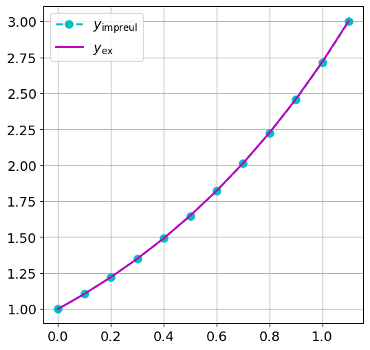
Example 15 (Implementation and testing of the improved Euler method)

We implement the improved explicit Euler from above and plot the analytical and the numerical solution. To determine the experimental order of convergence, we use again the compute_eoc function.

def compute_eoc(y0, t0, T, f, Nmax_list, solver, y_ex):
    errs = [ ]
    for Nmax in Nmax_list:
        ts, ys = solver(y0, t0, T, f, Nmax)
        ys_ex = y_ex(ts)
        errs.append(np.abs(ys - ys_ex).max())
        print("For Nmax = {:3}, max ||y(t_i) - y_i||= {:.3e}".format(Nmax,errs[-1]))

    errs = np.array(errs)
    Nmax_list = np.array(Nmax_list)
    dts = (T-t0)/Nmax_list

    eocs = np.log(errs[1:]/errs[:-1])/np.log(dts[1:]/dts[:-1])

    # Insert inf at beginning of eoc such that errs and eoc have same length 
    eocs = np.insert(eocs, 0, np.inf)

    return errs, eocs

Here is the implementation of the full example.

# Define Butcher table for improved Euler
a = np.array([[0,   0],
              [0.5, 0]])
b = np.array([0, 1])
c = np.array([0, 0.5])

# Create a new Runge Kutta solver
rk2 = ExplicitRungeKutta(a, b, c)

t0, T = 0, 1
y0 = 1
lam = 1
Nmax = 10

# rhs of IVP
f = lambda t,y: lam*y

# the solver can be simply called as before, namely as function:
ts, ys = rk2(y0, t0, T, f, Nmax)

plt.figure()
plt.plot(ts, ys, "c--o", label=r"$y_{\mathrm{impreul}}$")

# Exact solution to compare against
y_ex = lambda t: y0*np.exp(lam*(t-t0))

# Plot the exact solution (will appear in the plot above)
plt.plot(ts, y_ex(ts), "m-", label=r"$y_{\mathrm{ex}}$")
plt.legend()

# Run an EOC test
Nmax_list = [4, 8, 16, 32, 64, 128]

errs, eocs = compute_eoc(y0, t0, T, f, Nmax_list, rk2, y_ex)
print(errs)
print(eocs)

# Do a pretty print of the tables using panda

import pandas as pd
from IPython.display import display

table = pd.DataFrame({'Error': errs, 'EOC' : eocs})
display(table)

For Nmax =   4, max ||y(t_i) - y_i||= 2.343e-02
For Nmax =   8, max ||y(t_i) - y_i||= 6.441e-03
For Nmax =  16, max ||y(t_i) - y_i||= 1.688e-03
For Nmax =  32, max ||y(t_i) - y_i||= 4.322e-04
For Nmax =  64, max ||y(t_i) - y_i||= 1.093e-04
For Nmax = 128, max ||y(t_i) - y_i||= 2.749e-05
[2.34261385e-02 6.44058991e-03 1.68830598e-03 4.32154479e-04
 1.09316895e-04 2.74901378e-05]
[       inf 1.86285442 1.93161644 1.96595738 1.98303072 1.99153035]

	Error	EOC
0	0.023426	inf
1	0.006441	1.862854
2	0.001688	1.931616
3	0.000432	1.965957
4	0.000109	1.983031
5	0.000027	1.991530

While the term Runge-Kutta methods nowadays refer to the general scheme defined in Definition Definition 1: Runge-Kutta methods, particular schemes in the “early days” were named by their inventors, and there exists also the the classical 4-stage Runge-Kutta method which is defined by

\[\begin{split} \begin{array}{c|cccc} 0 & 0 & 0 & 0 & 0\\ \frac{1}{2} & \frac{1}{2} & 0 & 0 & 0\\ \frac{1}{2} & 0 & \frac{1}{2} & 0 & 0\\ 1 & 0 & 0 & 1 & 0 \\ \hline & \frac{1}{6} & \frac{1}{3} & \frac{1}{3} & \frac{1}{6} \end{array} \end{split}\]

a) Starting from this Butcher table, write down the explicit formulas for computing \(k_1,\ldots, k_4\) and \(y_{k+1}\).

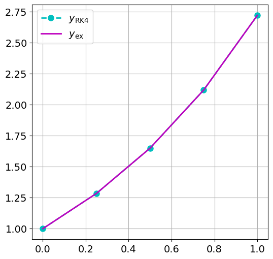
b) Build a solver based on the classical Runge-Kutta method using the ExplicitRungeKutta class and determine the convergence order experimentally.

# Insert your code here

# Define Butcher table for improved Euler
a = np.array([[0,   0,   0,  0],
              [1/2, 0,   0,  0],
              [0,   1/2, 0,  0],
              [0,   0,   1,  0]])
b = np.array([1/6, 1/3, 1/3, 1/6])
c = np.array([0, 1/2, 1/2, 1])

# Create a new Runge Kutta solver
rk4 = ExplicitRungeKutta(a, b, c)

t0, T = 0, 1
y0 = 1
lam = 1
Nmax = 4

# the solver can be simply called as before, namely as function:
ts, ys = rk4(y0, t0, T, f, Nmax)

plt.figure()
plt.plot(ts, ys, "c--o", label=r"$y_{\mathrm{RK4}}$")
plt.plot(ts, y_ex(ts), "m-", label=r"$y_{\mathrm{ex}}$")
plt.legend()

<matplotlib.legend.Legend at 0x7fa560ded8d0>

# Run an EOC test
Nmax_list = [4, 8, 16, 32, 64, 128]
errs, eocs = compute_eoc(y0, t0, T, f, Nmax_list, rk4, y_ex)
table = pd.DataFrame({'Error': errs, 'EOC' : eocs})
display(table)

For Nmax =   4, max ||y(t_i) - y_i||= 7.189e-05
For Nmax =   8, max ||y(t_i) - y_i||= 4.984e-06
For Nmax =  16, max ||y(t_i) - y_i||= 3.281e-07
For Nmax =  32, max ||y(t_i) - y_i||= 2.105e-08
For Nmax =  64, max ||y(t_i) - y_i||= 1.333e-09
For Nmax = 128, max ||y(t_i) - y_i||= 8.384e-11

	Error	EOC
0	7.188926e-05	inf
1	4.984042e-06	3.850388
2	3.281185e-07	3.925028
3	2.104785e-08	3.962472
4	1.332722e-09	3.981225
5	8.384093e-11	3.990577

Note

For the explicit Runge-Kutta methods, the \(s\times s\) matrix is in fact just a lower left triangle matrix, and often, the \(0\)s in the diagonal and upper right triangle are simply omitted. So, the Butcher table for the classical Runge-Kutta method reduces to

\[\begin{split} \begin{array}{c|cccc} 0 & & & & \\ \frac{1}{2} & \frac{1}{2} & & & \\ \frac{1}{2} & 0 & \frac{1}{2} & & \\ 1 & 0 & 0 & 1 & \\ \hline & \frac{1}{6} & \frac{1}{3} & \frac{1}{3} & \frac{1}{6} \end{array} \end{split}\]

Note

If \(f\) depends only on \(t\) but not on \(y\), the ODE \( y' = f(t, y) = f(t)\) reduces to a simpe integration problem, and in this case the classical Runge-Kutta methods reduces to the classical Simpson’s rule for numerical integration.

More generally, when applied to simple integration problems, Runge-Kutta methods reduces to various quadrature rules over the interval \( [t_i, t_{i+1}]\) with \(s\) quadrature points, where the integration points \(\{\xi_j\}_{i=1}^s\) and correspond weights \(\{w_i\}_{i=1}^s\) of the quadrature rules are given by respectively \(\xi_i = t_i + c_j\tau\), \(w_i = b_i\) for \(j=1,\ldots,s\)

See this wiki page for a list of various Runge-Kutta methods.

Runge-Kutta Methods via Numerical Integration

This section provides a supplemental and more in-depth motivation of how to arrive at the general concept of Runge-Kutta methods via numerical integration, similar to the ideas we already presented when we derived Crank-Nicolson, Heun’s method and the explicit trapezoidal rule.

For a given time interval \(I_i = [t_i, t_{i+1}]\) we want to compute \(y_{i+1}\) assuming that \(y_i\) is given. Starting from the exact expression

\[ y(t_{i+1}) - y(t_i) = \int_{t_i}^{t_{i+1}} y(t)'{\,\mathrm{d}t} = \int_{t_i}^{t_{i+1}} f(t, y(t)){\,\mathrm{d}t}, \]

the idea is now to approximate the integral by some quadrature rule \(\mathrm{Q}[\cdot](\{\xi_j\}_{j=1}^s,\{b_j\}_{j=1}^s)\) defined on \(I_i\). Then we get

\[ y(t_{i+1}) - y(t_i) = \int_{t_i}^{t_{i+1}} f(t, y(t)){\,\mathrm{d}t} \]

\[ \approx \tau \sum_{j=0}^s b_j f(\xi_j, y(\xi_j)) \]

Now we can define \(\{c_j\}_{j=1}^s\) such that \(\xi_j = t_{i} + c_j \tau\) for \(j=1,\ldots,s\)

Exercise 21 (A first condition on \(b_j\))

Question: What value do you expect for \(\sum_{j=1}^s b_{j}\)?

Choice A: \(\sum_{j=1}^s b_{j} = \tau\)

Choice B: \(\sum_{j=1}^s b_{j} = 0\)

Choice C: \(\sum_{j=1}^s b_{j} = 1\)

Solution to Exercise 21 (A first condition on \(b_j\))

The correct answer is C

In contrast to pure numerical integration, we don’t know the values of \(y(\xi_j)\). Again, we could use the same idea to approximate

\[ y(\xi_j) - y(t_i) =\int_{t_i}^{t_i+c_j \tau} y'(t){\,\mathrm{d}t} = \int_{t_i}^{t_i+c_j \tau} f(t, y(t)){\,\mathrm{d}t} \]

but then again we get a closure problem if we choose new quadrature points. The idea is now to not introduce even more new quadrature points but to use same \(y(\xi_j)\) to avoid the closure problem. Note that this leads to an approximation of the integrals \(\int_{t_i}^{t_i+c_j \tau}\) with possible nodes outside of \([t_i, t_i + c_j \tau ]\).

This leads us to

\[ y(\xi_j) - y(t_i) = \int_{t_i}^{t_i+c_j \tau} f(t, y(t)){\,\mathrm{d}t} \]

\[ \approx c_j \tau \sum_{l=1}^{s} \tilde{a}_{jl} f(\xi_l, y(\xi_l)) \]

\[ = \tau \sum_{l=1}^{s} {a}_{jl} f(\xi_l, y(\xi_l)) \]

where we set \( c_j \tilde{a}_{jl} = a_{jl}\).

Exercise 22 (A first condition on \(a_{jl}\))

Question: What value do you expect for \(\sum_{l=1}^s a_{jl}\)?

Choice A: \(\sum_{l=1}^s a_{jl} = \tfrac{1}{c_j}\)

Choice B: \(\sum_{l=1}^s a_{jl} = c_j \)

Choice C: \(\sum_{l=1}^s a_{jl} = 1 \)

Choice D: \(\sum_{l=1}^s a_{jl} = \tau \)

Solution to Exercise 22 (A first condition on \(a_{jl}\))

The correct answer is B

The previous discussion leads to the following alternative but equivalent definition of Runge-Kutta derivatives via stages \(Y_j\) (and not stage derivatives \(k_j\)):

Definition 8 (Runge-Kutta methods using stages \(\{Y_l\}_{l=1}^s\))

Given \(b_j\), \(c_j\), and \(a_{jl}\) for \(j,l = 1,\ldots s\), the Runge-Kutta method is defined by the recipe

\[\begin{align*} Y_{l} &:= y_i + \tau \sum_{j=1}^{s} {a}_{lj} f(t_i + c_j \tau, Y_j) \quad \text{for } l = 1,\ldots s, \\ y_{i+1} &:= y_i + \tau \sum_{j=1}^s b_j f(t_i + c_j \tau, Y_j) \end{align*}\]

Note that in the final step, all the function evaluation we need to perform have already been performed when computing \(Y_j\).

Therefore one often rewrite the scheme by introducing stage derivatives \(k_l\)

(19)\[\begin{align} k_j &:= f(t_i + c_j \tau, Y_j) \\ &= f(t_i + c_j \tau, y_i + \tau \sum_{l=1}^{s} {a}_{jl} k_l) \quad j = 1,\ldots s, \end{align}\]

so the resulting scheme will be

(20)\[\begin{align} k_{j} &:= f(t_i + c_j \tau, y_i + \tau \sum_{l=1}^{s} {a}_{jl} k_l) \quad j = 1,\ldots s, \\ y_{i+1} &:= y_{i} + \tau \sum_{j=1}^s b_j k_j \end{align}\]

which is exactly what we used as definition for general Runge-Kutta methods in the previous section.

Convergence of Runge-Kutta Methods

The convergence theorem for one-step methods gave us some necessary conditions to guarantee that a method is convergent order of \(p\): “consistency order \(p\)” + “Increment function satisfies a Lipschitz condition” \(\Rightarrow\) “convergence order \(p\).

``local truncation error behaves like \(\mathcal{O}(\tau^{p+1})\)”

• “Increment function satisfies a Lipschitz condition” \(\Rightarrow\) “global truncation error behaves like \(\mathcal{O}(\tau^{p})\)”

It turns out that for \(f\) is at least \(C^1\) with respect to all its arguments then the increment function \(\Phi\) associated with any Runge-Kutta methods satisfies a Lipschitz condition. The next theorem provides us a simple way to check whether a given Runge-Kutta (up to 4 stages) attains a certain consistency order.

Theorem 10 (Order conditions for Runge-Kutta methods)

Let the right-hand side \(f\) of an IVP be of \(C^p\). Then a Runge - Kutta method has consistency order \(p\) if and only if all the conditions up to and including \(p\) in the table below are satisfied.

\[\begin{split} \begin{array}{|c|c|c} \hline p & \text{conditions} \\ \hline 1 & \sum_{i=1}^s b_i = 1 \\ \hline 2 & \sum_{i=1}^s b_i c_i = 1/2 \\ \hline 3 & \sum_{i=1}^s b_i c_i^2 = 1/3\\ & \sum_{i,j=1}^s b_i a_{ij} c_j = 1/6 \\ \hline 4 & \sum_{i=1}^s b_ic_i^3=1/4 \\ & \sum_{i,j=1}^s b_i c_i a_{ij}c_j=1/8 \\ & \sum_{i,j=1}^s b_i a_{ij}c_j^2=1/12 \\ & \sum_{i,j,k=1}^s b_i a_{ij} a_{jk} c_k = 1/24 \\ \hline \end{array} \end{split}\]

where sums are taken over all the indices from 1 to \(s\).

Proof. We don’t present a proof, but the most straight-forward approach is similar to the way we show that Heun’s method and the improved Euler’s method are consistent of order 2: You perform a Taylor-expansion of the real solution and express all derivatives of \(y(t)\) in terms of derivatives of \(f\) by invoking the chain rule. Then you perform Taylor expansion of the various stages in the Runge-Kutta methods and gather all terms with the the same \(\tau\) order. To achieve a certain consistency order \(p\), the terms paired with \(\tau^k\), \(k=0,\ldots,p\) in the Taylor-expansion of the discrete solution must match the corresponding terms of the exact solution, which in turn will lead to certain condition for \(b_j, c_j\) and \(a_{ij}\).

Of course, this get quite cumbersome for higher order methods, and luckily there is a beautiful theory, will tells you how to do Taylor-expansion of the discrete and exact solution in term of derivatives of \(f\) in very structured manner. See [Hairer and Wanner, 1993](Chapter II.2).

Exercise 23 (Applying order conditions to Heun’s method)

Apply the conditions to Heun’s method, for which \(s=2\) and the Butcher tableau is

\[\begin{split} \begin{array}{c|cc} c_1 & a_{11} & a_{12} \\ c_2 & a_{21} & a_{22} \\ \hline & b_1 & b_2 \end{array} = \begin{array}{c|cc} 0 & 0 & 0 \\ 1 & 1 & 0 \\ \hline & \frac{1}{2} & \frac{1}{2} \end{array}. \end{split}\]

Solution to Exercise 23 (Applying order conditions to Heun's method)

The order conditions are:

\[\begin{align*} p&=1 & b_1 + b_2 &= \frac{1}{2} + \frac{1}{2}= 1 && \text{OK} \\ \\ \hline \\ p&=2 & b_1c_1 + b_2 c_2 &= \frac{1}{2}\cdot 0 + \frac{1}{2}\cdot 1 = \frac{1}{2} && \text{OK}\\ \\ \hline \\ p&=3 & b_1c_1^2 + b_2c_2^2 &= \frac{1}{2}\cdot 0^2 + \frac{1}{2}\cdot 1^2 = \frac{1}{2} \not= \frac{1}{3} && \text{Not satisfied} \\ & & b_1(a_{11}c_1+a_{12}c_2)+b_2(a_{21}c_1+a_{22}c_2) &= \frac{1}{2}(0\cdot0 + 0\cdot 1) + \frac{1}{2}(1\cdot 0 + 0\cdot 1) \\ &&&= 0 \not=\frac{1}{6} && \text{Not satisfied} \end{align*}\]

The method is of order 2.

Exercise 24 (Applying order conditions to the classical Runge-Kutta method)

In our numerical experiment earlier, we observed that classical 4-stage Runge-Kutta method defined by

\[\begin{split} \begin{array}{c|cccc} 0 & 0 & 0 & 0 & 0\\ \frac{1}{2} & \frac{1}{2} & 0 & 0 & 0\\ \frac{1}{2} & 0 & \frac{1}{2} & 0 & 0\\ 1 & 0 & 0 & 1 & 0 \\ \hline & \frac{1}{6} & \frac{1}{3} & \frac{1}{3} & \frac{1}{6} \end{array} \end{split}\]

had convergence order 4. Now use the order conditions to show, that this method indeed has consistency order 4.

Apply the conditions to Heun’s method, for which \(s=2\) and the Butcher tableau is

Theorem 11 (Convergence theorem for Runge-Kutta methods)

Given the IVP \({\boldsymbol y}' = {\boldsymbol f}(t, {\boldsymbol y}), {\boldsymbol y}(0) = {\boldsymbol y}_0\). Assume \(f \in C^p\) and that a given Runge-Kutta method satisfies the order conditions from Theorem 10 up to order \(p\). Then the Runge-Kutta method is convergent of order \(p\).

Proof. We only sketch the proof. First, the method has consistency order \(p\) thanks to the fullfilment of the order condition, Theorem 10. Thus, we only need to show that the increment function \(\Phi\) satisfies a Lipschitz condition. This can be achieved by employing a similar “bootstrapping” argument we used when proved that the increment function associated with the Heun’s method satisfies a Lipschitz condition.