Numerical integration: Interpolatory quadrature rules#
As usual we start by importing the some standard boilerplate code.
%matplotlib inline

import numpy as np
from numpy import pi
from math import sqrt
from numpy.linalg import solve, norm    # Solve linear systems and compute norms
import matplotlib.pyplot as plt
import matplotlib.cm as cm

newparams = {'figure.figsize': (10.0, 10.0),
             'axes.grid': True,
             'lines.markersize': 8,
             'lines.linewidth': 2,
             'font.size': 14}
plt.rcParams.update(newparams)
Introduction#
Imagine you want to compute the finite integral
The “usual” way is to find a primitive function \(F\) (also known as the indefinite integral of \(f\)) satisfying \(F'(x) = f(x)\) and then to compute
While there are many analytical integration techniques and extensive tables to determine definite integral for many integrands, more often than not it may not feasible or possible to compute the integral. For instance, what about
Finding the corresponding primitive is highly likely a hopeless endeavor. And sometimes there even innocent looking functions like \(e^{-x^2}\) for which there is not primitive functions which can expressed as a composition of standard functions such as \(\sin, \cos.\) etc.
A numerical quadrature or a quadrature rule is a formula for approximating such definite integrals \(I[f](a,b)\). Quadrature rules are usually of the form
where \(x_i\), \(w_i\) for \(i=0,1,\dotsc,n\) are respectively the nodes/points and the weights of the quadrature rule.
To emphasize that a quadrature rule is defined by some given quadrature points \(\{x_i\}_{i=0}^n\) and weights \(\{w_i\}_{i=0}^n\), we sometimes might write
If the function \(f\) is given from the context, we will for simplicity denote the integral and the quadrature simply as \(I(a,b)\) and \(Q(a,b)\).
Example 4 (Quadrature rules from previous math courses)
The trapezoidal rule, the midpoint rule and Simpson’s rule known from previous courses are all examples of numerical quadratures, and we quickly review them here, in addition to the very simple (and less accurate) left and right endpoint rules.
colors = plt.get_cmap("Pastel1").colors

def plot_qr_examples():
    f = lambda x : np.exp(x)
    fig, axs = plt.subplots(2,2)
    fig.set_figheight(8)
    # fig.set_figwidth(8)
    fig.set_figwidth(fig.get_size_inches()[0]*1.5)
    #axs[0].add_axes([0.1, 0.2, 0.8, 0.7])
    a, b = -0.5,0.5
    l, r = -1.0, 1.0
    x_a = np.linspace(a, b, 100)

    for raxs in axs:
        for ax in raxs:
            ax.set_xlim(l, r)
            x = np.linspace(l, r, 100)
            ax.plot(x, f(x), "k--", label="$f(x)$")
            ax.fill_between(x_a, f(x_a), alpha=0.1, color='k')
            ax.xaxis.set_ticks_position('bottom')
            ax.set_xticks([a,b])
            ax.set_xticklabels(["$a$", "$b$"])
            ax.set_yticks([])
            ax.legend(loc="upper center")

    # Left endpoint rule
    axs[0,0].bar(a, f(a), b-a, align='edge', color=colors[0])
    axs[0,0].plot(a,f(a), 'ko', markersize="12")
    axs[0,0].set_title("Left endpoint rule")
    axs[0,0].annotate('$f(a)$',
             xy=(a, f(a)), xytext=(-10, 10),
             textcoords="offset points")

    # Right endpoint rule
    axs[0,1].bar(a, f(b), b-a, align='edge',  color=colors[1])
    axs[0,1].plot(b,f(b), 'ko', markersize="15")
    axs[0,1].set_title("Right endpoint rule")
    axs[0,1].annotate('$f(b)$',
             xy=(b, f(b)), xytext=(-10, 10),
             textcoords="offset points")
    # Midpoint rule
    axs[1,0].bar(a, f((a+b)/2), b-a, align='edge', color=colors[2])
    axs[1,0].plot((a+b)/2,f((a+b)/2), 'ko', markersize="15")
    axs[1,0].set_title("Midpoint rule")
    axs[1,0].annotate('$f((a+b)/2))$',
             xy=((a+b)/2, f((a+b)/2)), xytext=(-10, 10),
             textcoords="offset points")

    # Trapezoidal rule
    axs[1,1].set_title("Trapezoidal rule")
    axs[1,1].fill_between([a,b], [f(a), f(b)], alpha=0.8, color=colors[4])
    axs[1,1].plot([a,b],f([a,b]), 'ko', markersize="15")
    axs[1,1].annotate('$f(a)$',
             xy=(a, f(a)), xytext=(-10, 10),
             textcoords="offset points")
    axs[1,1].annotate('$f(b)$',
             xy=(b, f(b)), xytext=(-10, 10),
             textcoords="offset points")
    axs[1,1].annotate('$f(b)$',
             xy=(b, f(b)), xytext=(-10, 10),
             textcoords="offset points")
plot_qr_examples()
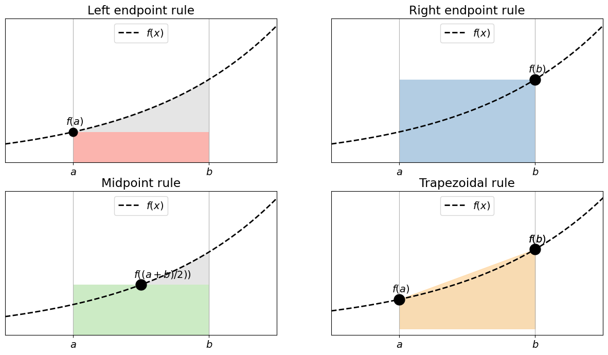
Left and right endpoint rule are among the simplest possible quadrature rule defined by
respectively. The (single) quadrature point for \(QL[\cdot]\) and \(QR[\cdot]\) is given by \(x_0 = a\) and \(x_0 = b\) respectively, and both use the corresponding weight \(w_0 = b-a\).
Midpoint rule is the quadrature rule defined by
The node is given by the midpoint, \(x_0 = \tfrac{a+b}{2}\) with the corresponding weight \(w_0 = b-a\).
Trapezoidal rule is given by
and thus the nodes are defined by \(x_0 = a\), \(x_1 = b\) with corresponding weights \(w_0 = w_1 = \tfrac{b-a}{2}\).
Finally, Simpson’s rule which you know from Matte 1, is defined as follows:
which we identify as quadrature rule with 3 points \(x_0 = a, x_1 = \tfrac{a+b}{2}, x_2 = b\) and corresponding weights \(w_0 = w_2 = \tfrac{b-a}{6}\) and \(w_1 = \tfrac{4(b-a)}{6}\).
In this note we will see how quadrature rules can be constructed from integration of interpolation polynomials. We will demonstrate how to do error analysis and how to find error estimates.
Quadrature based on polynomial interpolation.#
This section relies on the content of the note on polynomial interpolation, in particular the section on Lagrange polynomials.
Choose \(n+1\) distinct nodes \(x_i\), \(i=0,\dotsc,n\) in the interval \([a,b]\), and let \(p_n(x)\) be the interpolation polynomial satisfying the interpolation condition
We will then use \(\int_a^b p_n(x){\,\mathrm{d}x}\) as an approximation to \(\int_a^b f(x){\,\mathrm{d}x}\). By using the Lagrange form of the polynomial
with the cardinal functions \(\ell_i(x)\) given by
the following quadrature formula is obtained
where the weights in the quadrature are simply the integral of the cardinal functions over the interval
Let us derive three schemes for integration over the interval \([0,1]\), which we will finally apply to the integral
Example 5 (The trapezoidal rule revisited)
Let \(x_0=0\) and \(x_1=1\). The cardinal functions and thus the weights are given by
and the corresponding quadrature rule is the trapezoidal rule (usually denoted by \(T\)) recalled in exa-known-qr-rules with \([a,b] = [0,1]\):
Example 6 (Gauß-Legendre quadrature for \(n=2\))
Let \(x_0=1/2 + \sqrt{3}/6\) and \(x_1 = 1/2 - \sqrt{3}/6\). Then
The quadrature rule is
Example 7 (Simpson’s rule revisited)
We construct Simpson’s rule on the interval \([0,1]\) by choosing the nodes \(x_0=0\), \(x_1=0.5\) and \(x_2=1\). The corresponding cardinal functions are
which gives the weights
such that
Exercise 7 (Accuracy of some quadrature rules)
Use the QR function below
to compute an approximate value of integral for \(f(x)= \cos\left(\frac{\pi}{2}x\right)\)
using the quadrature rules from exa-trap-rule-revist-exa-simpson-rule. Tabulate the corresponding quadrature errors \(I[f](0,1) - Q[f](0,1)\).
def QR(f, xq, wq):
    """ Computes an approximation of the integral f
    for a given quadrature rule.

    Input:
        f:  integrand
        xq: list of quadrature nodes
        wq: list of quadrature weights
    """
    n = len(xq)
    if (n != len(wq)):
        raise RuntimeError("Error: Need same number of quadrature nodes and weights!")
    return np.array(wq)@f(np.array(xq))
Hint. You can start with (fill in values for any \(\ldots\))
# Define function
def f(x):
    return ...

# Exact integral
int_f = 2/pi

# Trapezoidal rule
xq = ...
wq = ...

qr_f = ...
print("Q[f] = {}".format(qr_f))
print("I[f] - Q[f] = {:.10e}".format(int_f - qr_f))
# Insert your code here.
Solution to Exercise 7 (Accuracy of some quadrature rules)
# Define function
def f(x):
    return np.cos(pi/2*x)

# Exact integral
int_f = 2.0/pi
print("I[f] = {}".format(int_f))

# Trapezoidal
xq = [0,1]
wq = [0.5, 0.5]

qr_f = QR(f, xq, wq)
print("Error for the trapezoidal rule")
print("Q[f] = {}".format(qr_f))
print("I[f] - Q[f] = {:.10e}".format(int_f - qr_f))

# Gauss-Legendre
print("Error for Gauss-Legendre")
xq = [0.5-sqrt(3)/6, 0.5+sqrt(3)/6]
wq = [0.5, 0.5]

qr_f = QR(f, xq, wq)
print("Q[f] = {}".format(qr_f))
print("I[f] - Q[f] = {:.10e}".format(int_f - qr_f))

# Simpson
print("Error for Simpson")
xq = [0, 0.5, 1]
wq = [1/6., 4/6., 1/6.]

qr_f = QR(f, xq, wq)
print("Q[f] = {}".format(qr_f))
print("I[f] - Q[f] = {:.10e}".format(int_f - qr_f))
I[f] = 0.6366197723675814
Error for the trapezoidal rule
Q[f] = 0.5
I[f] - Q[f] = 1.3661977237e-01
Error for Gauss-Legendre
Q[f] = 0.6356474078605917
I[f] - Q[f] = 9.7236450699e-04
Error for Simpson
Q[f] = 0.6380711874576983
I[f] - Q[f] = -1.4514150901e-03
Remark 2
We observe that with the same number of quadrature points, the Gauß-Legendre quadrature gives a much more accurate answer then the trapezoidal rule. So the choice of nodes clearly matters. Simpon’s rule gives very similar results to Gauß-Legendre quadrature, but it uses 3 instead of 2 quadrature nodes. The quadrature rules which based on polynomial interpolation and equidistributed quadrature nodes go under the name Newton Cotes formulas (see below).
Degree of exactness and an estimate of the quadrature error#
Motivated by the previous examples, we know take a closer look at how assess the quality of a method. We start with the following definition.
Definition 3 (The degree of exactness (presisjonsgrad))
A numerical quadrature has degree of exactness \(d\) if \(Q[p](a,b) = I[p](a,b)\) for all \(p \in \mathbb{P}_d\) and there is at least one \(p\in \mathbb{P}_{d+1}\) such that \(Q[p](a,b) \not= I[p](a,b)\).
Since both integrals and quadratures are linear in the integrand \(f\), the degree of exactness is \(d\) if
Observation 4
All quadratures constructed from Lagrange interpolation polynomials in \(n+1\) distinct nodes will automatically have a degree of exactness of at least \(n\). This follows immediately from the fact the interpolation polynomial \(p_n \in \mathbb{P}_n\) of any polynomial \(q \in \mathbb{P}_n\) is just the original polynomial \(q\) itself. But sometimes the degree of exactness can be even higher as the next exercise shows!
Exercise 8 (Degree of exactness for some quadrature rules)
What is the degree of exactness for the left and right endpoint rule from exa-known-qr-rules?
What is the degree of exactness for the trapezoidal and midpoint rule from exa-known-qr-rules?
What is the degree of exactness for Gauß-Legendre quadrature for 2 points from exa:gauss-legend-quad?
What is the degree of exactness for Simpson’s rule from exa-simpson-rule?
We test the degree of exactness for each of theses quadratures by
computing the exact integral \(I[x^n](0,1) = \int_0^1 x^n dx\) for let’s say \(n=0,1,2,3,4\)
computing the corresponding numerical integral \(Q[x^n](0,1)\) using the given quadrature rule.
look at the difference \(I[x^n](0,1) - Q[x^n](0,1)\) for each of the quadrature rules.
You can start from the code outline below.
Hint. You can do this either using pen and paper (boring!) or numerically (more fun!), using the code from Exercise 7, see the code outline below.
from collections import namedtuple
qr_tuple = namedtuple("qr_tuple", ["name", "xq", "wq"])

quadrature_rules =  [
    qr_tuple(name = "left endpoint rule", xq=[0], wq=[1]),
    qr_tuple(name = "right endpoint rule", xq=[1], wq=[1])
]
print(quadrature_rules)

# n defines maximal monomial powers you want to test
for n in range(5):

    print("===========================================")
    print(f"Testing degree of exactness for n = {n}")

    # Define function
    def f(x):
        return x**n

    # Exact integral
    int_f = 1./(n+1)

    for qr in quadrature_rules:
        print("-------------------------------------------")
        print(f"Testing {qr.name}")

        qr_f = QR(f, qr.xq, qr.wq)
        print(f"Q[f] = {qr_f}")
        print(f"I[f] - Q[f] = {int_f - qr_f:.16e}")
# Insert your code here
It is mentimeter time! Let’s go to https://www.menti.com/ for a little quiz.
Observation 5
(Will be updated after the mentimeter!)
left and right end point rule have degree of exactness = 0
mid point rule has degree of exactness = 1
trapezoidal rule has degree of exactness = 1
Gauß-Legendre rule has degree of exactness = 3
Simpson rule has degree of exactness = 3
Estimates for the quadrature error#
Theorem 4 (Error estimate for quadrature rule with degree of exactness \(n\))
Assume that \(f \in C^{n+1}(a,b)\) and let \(Q[\cdot](\{x_i\}_{i=0}^n, \{w_i\}_{i=0}^n)\) be a quadrature rule which has degree of exactness \(n\). Then the quadrature error \(|I[f]-Q[f]|\) can be estimated by
where \(M=\max_{\xi \in [a,b]} |f^{n+1}(\xi)|\).
Proof. Let \(p_n \in \mathbb{P}_n\) be the interpolation polynomial satisfying \(p_n(x_i) = f(x_i)\) for \(i=0,\ldots,n\). Thanks to the error estimate for the interpolation error, we know that
for some \(\xi(x) \in (a,b)\). Since \(Q(a,b)\) has degree of exactness \(n\) we have \(I[p_n] = Q[p_n] = Q[f]\) and thus
which concludes the proof.
The advantage of the previous theorem is that it is easy to prove. On downside is that the provided estimate can be rather crude, and often sharper estimates can be established. We give two examples here of some sharper estimates (but without proof).
Theorem 5 (Error estimate for the trapezoidal rule)
For the trapezoidal rule, there is a \(\xi \in (a,b)\) such that
Theorem 6 (Error estimate for Simpson’s rule)
For Simpson’s rule, there is a \(\xi \in (a,b)\) such that
Newton-Cotes formulas#
We have already seen that given \(n+1\) distinct but otherwise arbitrary quadrature nodes \(\{x_i\}_{i=0}^n \subset [a,b]\), we can construct a quadrature rule \( \mathrm{Q}[\cdot](\{x_i\}_{i=0}^{n+1},\{w_i\}_{i=0}^{n+1}) \) based on polynomial interpolation which has degree of exactness equals to \(n\).
An classical example was the trapezoidal rule, which are based on the two quadrature points \(x_0=a\) and \(x_1=b\) and which has degree of exactness equal to \(1\).
The trapezoidal is the simplest example of a quadrature formula which belongs to the so-called Newton Cotes formulas.
By definition, Newton-Cotes formulas are quadrature rules which are based on equidistributed nodes \(\{x_i\}_{i=0}^n \subset [a,b]\) and have degree of exactness equals to \(n\).
The simplest choices here — the closed Newton-Cotes methods — use the nodes \(x_i = a + ih\) with \(h = (b-a)/n\). Examples of these are the Trapezoidal rule and Simpson’s rule. The main appeal of these rules is the simple definition of the nodes.
If \(n\) is odd, the Newton-Cotes method with \(n+1\) nodes has degree of precision \(n\); if \(n\) is even, it has degree of precision \(n+1\). The corresponding convergence order for the composite rule is, as for all such rules, one larger than the degree of precision, provided that the function \(f\) is sufficiently smooth.
However, for \(n \ge 8\) negative weights begin to appear in the definitions. Note that for a positive function \(f(x) \geqslant 0\) we have that the integral \(I[f](a,b) \geqslant 0\) But for a quadrature rule with negative weights we have not necessarily that \(Q[f](a,b) \geqslant 0\)! This has the undesired effect that the numerical integral of a positive function can be negative.
In addition, this can lead to cancellation errors in the numerical evaluation, which may result in a lower practical accuracy. Since the rules with \(n=6\) and \(n=7\) yield the same convergence order, this mean that it is mostly the rules with \(n \le 6\) that are used in practice.
The open Newton-Cotes methods, in contrast, use the nodes \(x_i = a + (i+1/2)h\) with \(h = (b-a)/(n+1)\). The simplest example here is the midpoint rule. Here negative weights appear already for \(n \ge 2\). Thus the midpoint rule is the only such rule that is commonly used in applications.