Numerical differentiation and spectral derivatives#
%matplotlib inline
import numpy as np
import matplotlib.pyplot as plt
from scipy.fft import fft, fft2, ifft, ifft2, fftfreq, fftshift
import pandas as pd
Assume we have a function \(f \in C_p^k(0,L)\) (the space of \(k\) times continuously differentiable, \(L\)-period functions).
Given a set of \(N\) equi-distributed sampling points \(x_l = l N/L, l =0,\ldots, N-1\) with distance \(h = N/L\), we denote by \(\boldsymbol{f} = \{f(x_l)\}_{l=0}^{N-1} \in \mathbb{R}^N\) the corresponding vector of the samples of \(f\) and write \(\boldsymbol{f}(l) = f(x_l)\).
Let’s consider the following 4 ways to approximate the derivative of \(f\) at \(x_l\):
Here \(\mathbf{k}\) is the wave number vector \(2\pi/L (0,1,\ldots,N/2-1,-N/2,-N/2+1,\ldots,-1)\),
Aproximation properties of the finite difference operators#
Proposition 1
Assuming that the function \(f\) is sufficiently differentiable, the following estimates hold:
for \(h \to 0\) (respectively \(N \to \infty\)).
Proof. The proof is based on the Taylor expansion of the function \(f\) around the point \(x_k\).
Forward difference: Using Taylor expansion around \(x_l\):
\[ f(x_{l+1}) = f(x_l) + h f'(x_l) + \frac{h^2}{2} f''(x_l) + \mathcal{O}(h^3) \]Therefore,\[ \partial^+ f(x_l) = \frac{f(x_{l+1}) - f(x_l)}{h} = f'(x_l) + \frac{h}{2} f''(x_l) + \mathcal{O}(h^2) \]Hence,\[ \partial^+ f(x_l) - f'(x_l) = \frac{h}{2} f''(x_l) + \mathcal{O}(h^2) = \mathcal{O}(h) \]Backward difference: Using Taylor expansion around \(x_l\):
\[ f(x_{l-1}) = f(x_l) - h f'(x_l) + \frac{h^2}{2} f''(x_l) - \mathcal{O}(h^3) \]Therefore,\[ \partial^- f(x_l) = \frac{f(x_l) - f(x_{l-1})}{h} = f'(x_l) -\frac{h}{2} f''(x_l) + \mathcal{O}(h^2) \]Hence,\[ \partial^- f(x_l) - f'(x_l) = \frac{h}{2} f''(x_l) + \mathcal{O}(h^2) = \mathcal{O}(h) \]Central difference: Using Taylor expansion around \(x_l\):
\[ f(x_{l+1}) = f(x_l) + h f'(x_l) + \frac{h^2}{2} f''(x_l) + \frac{h^3}{6} f'''(x_l) + \mathcal{O}(h^4) \]\[ f(x_{l-1}) = f(x_l) - h f'(x_l) + \frac{h^2}{2} f''(x_l) - \frac{h^3}{6} f'''(x_l) + \mathcal{O}(h^4) \]Therefore,\[ \partial^\circ f(x_l) = \frac{f(x_{l+1}) - f(x_{l-1})}{2h} = f'(x_l) + \mathcal{O}(h^2) \]Hence,\[ \partial^\circ f(x_l) - f'(x_l) = \mathcal{O}(h^2) \]
Numerical experiments#
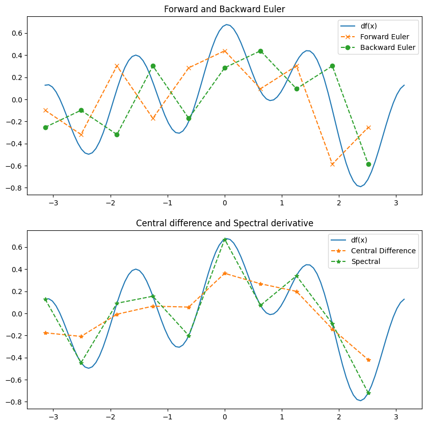
Next, we implement the 4 numerical differentiation methods and compare their performance on the functions
First, for four different sampleing sizes \(N = 4, 8, 12, 16\), plot the exact derivate \(f'(x)\) and the corresponding 4 different approximations. Afterward, perform a convergence study of the error of the various numerical differentiation methods, for \(N = 4, 8, 12, 16, 20, 24, 28, 32, 36\) and tabulate the error and the convergence rate of the numerical differentiation methods. Discuss the results and estimate theoretically based on your tabulated values, how large \(N\) should be chosen so that the forward/backward/central finite differences obtain a given accuracy as the spectral derivative for \(N=24\).
# Forward Euler
def df_forward(f, x):
    dx = x[1] - x[0]
    df = np.zeros_like(x)
    df[:-1] = (f(x[1:]) - f(x[:-1]))/dx
    df[-1] = (f(x[0]) - f(x[-1]))/dx
    return df

# Backward Euler
def df_backward(f, x):
    dx = x[1] - x[0]
    df = np.zeros_like(x)
    df[1:] = (f(x[1:]) - f(x[:-1]))/dx
    df[0] = (f(x[0]) - f(x[-1]))/dx
    return df

# Central difference
def df_central(f, x):
    dx = x[1] - x[0]
    df = np.zeros_like(x)
    df[1:-1] = (f(x[2:]) - f(x[:-2]))/(2*dx)
    df[0] = (f(x[1]) - f(x[-1]))/(2*dx)
    df[-1] = (f(x[0]) - f(x[-2]))/(2*dx)
    return df

# Very important:
# Use arange instead of linspace to obtain half-open intervals
# This is important since we have periodic boundary conditions!
def df_spectral(f, x):
    # You can either do
    # f_hat = fft(f(x))
    # N, dx = len(x), (x[1] - x[0])
    # k = fftfreq(N, d=dx)*2*np.pi
    # df_hat = 1j * k * f_hat
    # df = ifft(df_hat).real
    # return df
    # ... or write a one-liner
    return ifft(1j*fftfreq(len(x), (x[1] - x[0])/(2*np.pi))*fft(f(x))).real
L = 2*np.pi
# L = np.pi
N = 10
dx = L/N
# Note that we do not need to include the last point
# due to the periodic boundary conditions
x = np.arange(-L/2, L/2, dx)
# Define a function and its derivative
# f = lambda x: np.cos(x) + 0.5*np.sin(4*x)
# df = lambda x: -np.sin(x) + 0.4*np.cos(4*x)
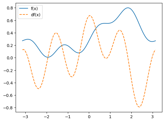
f = lambda x: 0.1*np.exp(1+np.sin(x)) + 0.1*np.sin(4*x)
df = lambda x: 0.1*np.cos(x)*np.exp(1+np.sin(x)) + 0.4*np.cos(4*x)
xfine = np.linspace(-L/2, L/2, 10*N)
# plt.figure(figsize=(10, 6))
plt.plot(xfine, f(xfine), label='f(x)')
plt.plot(xfine, df(xfine), "--", label='df(x)')
plt.legend()
plt.show()
fig, axes = plt.subplots(2, 1, figsize=(10, 10))

# First subplot: df, Forward Euler, Backward Euler
axes[0].plot(xfine, df(xfine), label='df(x)')
axes[0].plot(x, df_forward(f, x),  "--x", label='Forward Euler')
axes[0].plot(x, df_backward(f, x), "--o", label='Backward Euler')
axes[0].legend()
axes[0].set_title('Forward and Backward Euler')

# Second subplot: df, Central Euler, Spectral
axes[1].plot(xfine, df(xfine), label='df(x)')
axes[1].plot(x, df_central(f, x),  "--*", label='Central Difference')
axes[1].plot(x, df_spectral(f, x),  "--*", label='Spectral')
axes[1].legend()
axes[1].set_title('Central difference and Spectral derivative')

plt.show()
f = lambda x: np.exp(1+np.sin(x))
df = lambda x: np.cos(x)*np.exp(1+np.sin(x))

# Try this one afterwards
# f = lambda x: np.sin(x)
# df = lambda x: np.cos(x)

def compute_eoc(f, df, L, N_list, df_num):
    errs = []
    for N in N_list:
        dx = L/N
        x = np.arange(-L/2, L/2, dx)
        errs.append(np.abs( df(x) - df_num(f, x), np.inf).max())
        # print(f'N = {N}, error = {errs[-1]}')
    errs = np.array(errs)
    N_list = np.array(N_list)
    eocs = np.log(errs[1:]/errs[:-1])/np.log(N_list[:-1]/N_list[1:])
    eocs = np.insert(eocs, 0, np.inf)
    return errs, eocs

N_list = [4 + 4*k for k in range(0,9)]
print(N_list)
[4, 8, 12, 16, 20, 24, 28, 32, 36]
table = pd.DataFrame(index=N_list)
for method in [df_forward, df_backward, df_central, df_spectral]:
    errs, eocs = compute_eoc(f, df, L, N_list, method)
    table[method.__name__ + " err"] = errs
    table[method.__name__ + " eoc"] = eocs

display(table)
---------------------------------------------------------------------------
TypeError                                 Traceback (most recent call last)
Cell In[6], line 3
      1 table = pd.DataFrame(index=N_list)
      2 for method in [df_forward, df_backward, df_central, df_spectral]:
----> 3     errs, eocs = compute_eoc(f, df, L, N_list, method)
      4     table[method.__name__ + " err"] = errs
      5     table[method.__name__ + " eoc"] = eocs

Cell In[5], line 13, in compute_eoc(f, df, L, N_list, df_num)
     11     dx = L/N
     12     x = np.arange(-L/2, L/2, dx)
---> 13     errs.append(np.abs( df(x) - df_num(f, x), np.inf).max())
     14     # print(f'N = {N}, error = {errs[-1]}')
     15 errs = np.array(errs)

TypeError: return arrays must be of ArrayType
Discussion.
The forward and backward difference operators have a first order convergence rate, while the central difference operator has a second order convergence rate. This can be clearly seen in the convergence study, where double the number of sampling points reduces the error by a factor of 4 for the central difference operator, but only by a factor of 2 for the forward and backward difference operators.
The spectral derivative has a much higher convergence rate than the finite difference operators. For \(N=28\), the error of the spectral derivative is already roughly at machine precisison. Consequently, the error of the spectral derivative cannot get smaller for N roughly larger than 24, which is why we don’t observe any positive convergence rate for \(N>28\).