Numerical solution of ordinary differential equations: Euler’s and Heun’s method#
As always we start by running some necessary boilerplate code.
import numpy as np
import matplotlib.pyplot as plt
import matplotlib.cm as cm

newparams = {'figure.figsize': (6.0, 6.0),
             'axes.grid': True,
             'lines.markersize': 8,
             'lines.linewidth': 2,
             'font.size': 14}
plt.rcParams.update(newparams)
Euler’s method#
Now we turn to our first numerical method, namely Euler’s method, known from Mathematics 1. We quickly review two alternative derivations, namely one based on numerical differentiation and one on numerical integration.
Derivation of Euler’s method.
Euler’s method is the simplest example of a so-called one step method (OSM). Given the IVP
and some final time \(T\), we want to compute an approximation of \(y(t)\) on \([t_0, T]\).
We start from \(t_0\) and choose some (usually small) time step size \(\tau_0\) and set the new time \(t_1 = t_0 + \tau_0\). The goal is to compute a value \(y_1\) serving as approximation of \(y(t_1)\).
To do so, we Taylor expand the exact (but unknown) solution \(y(t_0+\tau)\) around \(x_0\):
Assume the step size \(\tau\) to be small such that the solution is dominated by the first two terms. In that case, these can be used as the numerical approximation in the next step \(t_1 := t_0 + \tau\):
which means we compute
as an approximation to \(y(t_1)\)
Now we can repeat this procedure and choose the next (possibly different) time step \(\tau_1\) and compute a numerical approximation \(y_2\) for \(y(t)\) at \(t_2 = t_1 + \tau_1\) by setting
The idea is to repeat this procedure until we reached the final time \(T\) resulting in the following
Algorithm 1 (Euler’s method)
Input Given a function \(f(t,y)\), initial value \((t_0,y_0)\) and maximal number of time steps \(N\).
Output Array \(\{(t_k, y_k)\}_{k=0}^{N}\) collecting approximate function value \(y_k \approx y(t_k)\).
Set \(t = t_0\).
\(\texttt{while } t < T\):
Choose \(\tau\)
\(\displaystyle y_{k+1} := y_{k} + \tau f(t_k, y_k)\)
\(t_{k+1}:=t_k+\tau_k\)
\(t := t_{k+1}\)
So we can think of the Euler method as a method which approximates the continuous but unknown solution \(y(t): [t_0, T] \to \mathbb{R}\) by a discrete function \(y_{\Delta}:\{t_0, t_1, \ldots, t_{N_t}\}\) such that \(y_{\Delta}(t_k) := y_k \approx y(t_k)\).
How to choose \(\tau_i\)? The simplest possibility is to set a maximum number of steps \(N_{\mathrm{max}} = N_t\) and then to chose a constant time step \(\tau = (T-t_0)/N_{\mathrm{max}}\) resulting in \(N_{\mathrm{max}}+1\) equidistributed points. Later we will also learn, how to choose the time step adaptively, depending on the solution’s behavior.
Also, in order to compute an approximation at the next point \(t_{k+1}\), Euler’s method only needs to know \(f\), \(\tau_k\) and the solution \(y_k\) at the current point \(t_k\), but not at earlier points \(t_{k-1}, t_{k-2}, \ldots\) Thus Euler’s method is an prototype of a so-called One Step Method (OSM). We will formalize this concept later.
Numerical solution between the nodes.
At first we have only an approximation of \(y(t)\) at the \(N_t +1 \) nodes \(y_{\Delta}:\{t_0, t_1, \ldots, t_{N_t}\}\). If we want to evaluate the numerical solution between the nodes, a natural idea is to extend the discrete solution linearly between each pair of time nodes \(t_{k}, t_{k+1}\). This is compatible with the way the numerical solution can be plotted, namely by connected each pair \((t_k, y_k)\) and \((t_{k+1}, y_{k+1})\) with straight lines.
Interpretation: Euler’s method via forward difference operators.
After rearranging terms, we can also interpret the computation of an approximation \(y_1 \approx y(t_1)\) as replacing the derivative \(y'(t_0) = f(t_0, y_0)\) with a forward difference operator
Thus Euler’s method replace the differential quotient by a difference quotient.
Alternative derivation via numerical integration. Recall that for a function \(f: [a,b] \to \mathbb{R}\), we can approximate its integral \(\int_a^b f(t) {\,\mathrm{d}t}\) using a very simple left endpoint quadrature rule from Example 4,
Turning to our IVP, we now formally integrate the ODE \(y'(t) = f(t, y(t))\) on the time interval \(I_k = [t_k, t_{k+1}]\) and then apply the left endpoint quadrature rule to obtain
Sorting terms gives us back Euler’s method
Implementation of Euler’s method#
Euler’s method can be implemented in only a few lines of code:
def explicit_euler(y0, t0, T, f, Nmax):
    ys = [y0]
    ts = [t0]
    dt = (T - t0)/Nmax
    while(ts[-1] < T):
        t, y = ts[-1], ys[-1]
        ys.append(y + dt*f(t, y))
        ts.append(t + dt)
    return (np.array(ts), np.array(ys))
Let’s test Euler’s method with the simple IVP given in Example 8.
t0, T = 0, 1
y0 = 1
lam = 1
Nmax = 4

# rhs of IVP
f = lambda t,y: lam*y
print(f(t0, y0))

# Compute numerical solution using Euler
ts, ys_eul = explicit_euler(y0, t0, T, f, Nmax)

# Exact solution to compare against
y_ex = lambda t: y0*np.exp(lam*(t-t0))
ys_ex = y_ex(ts)
1
# Plot it
plt.figure()
plt.plot(ts, ys_ex, 'b-o')
plt.plot(ts, ys_eul, 'r--o')
plt.legend(["$y_{ex}$", "$y_{eul}$" ])
<matplotlib.legend.Legend at 0x7f98b0492350>
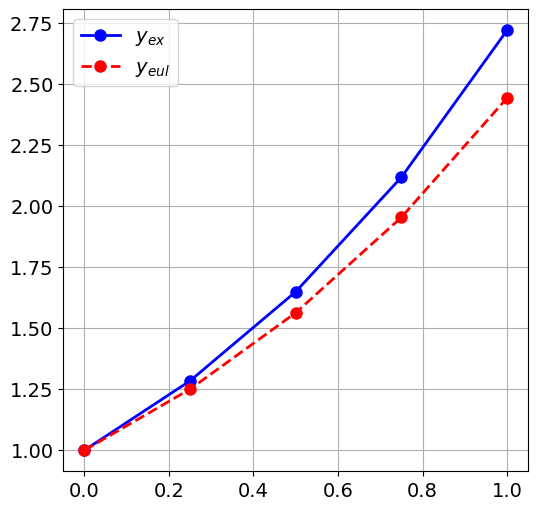
Plot the solution for various \(N_t\), say \(N_t = 4, 8, 16, 32\) against the exact solution given in Example 8.
Exercise 12 (Error study for the Euler’s method)
We observed that the more we decrease the constant step size \(\tau\) (or increase \(N_{\mathrm{max}}\)), the closer the numerical solution gets to the exact solution.
Now we ask you to quantify this. More precisely, write some code to compute the error
for \(N_{\mathrm{max}} = 4, 8, 16, 32, 64, 128\). How does the error reduces if you double the number of points?
Complete the following code outline by filling in the missing
code indicated by ....
def error_study(y0, t0, T, f, Nmax_list, solver, y_ex):
    """
    Performs an error study for a given ODE solver by computing the maximum error
    between the numerical solution and the exact solution for different values of Nmax.
    Print the list of error reduction rates computed from two consecutively solves.

    Parameters:
      y0 : Initial condition.
      t0 : Initial time.
      T (float): Final time.
      f (function): Function representing the ODE.
      Nmax_list (list of int): List of maximum number of steps to use in the solver.
      solver (function): Numerical solver function.
      y_ex (function): Exact solution function.

    Returns:
      None
    """
    max_errs = []
    for Nmax in Nmax_list:
        # Compute list of timestep ts and computed solution ys
        ts, ys = ...
        # Evaluate y_ex in ts
        ys_ex = ...
        # Compute max error for given solution and print it
        max_errs.append(...)
        print(f"For Nmax = {Nmax:3}, max ||y(t_i) - y_i||= {max_errs[-1]:.3e}")
    # Turn list into array to allow for vectorized division
    max_errs = np.array(max_errs)
    rates = ...
    print("The computed error reduction rates are")
    print(rates)


# Define list for N_max and run error study
Nmax_list = [4, 8, 16, 32, 64, 128]
error_study(y0, t0, T, f, Nmax_list, explicit_euler, y_ex)
# Insert code here
Solution to Exercise 12 (Error study for the Euler's method)
def error_study(y0, t0, T, f, Nmax_list, solver, y_ex):
    max_errs = []
    for Nmax in Nmax_list:
        ts, ys = solver(y0, t0, T, f, Nmax)
        ys_ex = y_ex(ts)
        errors = ys - ys_ex
        max_errs.append(np.abs(errors).max())
        print(f"For Nmax = {Nmax:3}, max ||y(t_i) - y_i||= {max_errs[-1]:.3e}")
    max_errs = np.array(max_errs)
    rates = max_errs[:-1]/max_errs[1:]
    print("The computed error reduction rates are")
    print(rates)

Nmax_list = [4, 8, 16, 32, 64, 128]
error_study(y0, t0, T, f, Nmax_list, explicit_euler, y_ex)
For Nmax =   4, max ||y(t_i) - y_i||= 2.769e-01
For Nmax =   8, max ||y(t_i) - y_i||= 1.525e-01
For Nmax =  16, max ||y(t_i) - y_i||= 8.035e-02
For Nmax =  32, max ||y(t_i) - y_i||= 4.129e-02
For Nmax =  64, max ||y(t_i) - y_i||= 2.094e-02
For Nmax = 128, max ||y(t_i) - y_i||= 1.054e-02
The computed error reduction rates are
[1.81560954 1.89783438 1.94599236 1.97219964 1.98589165]
Heun’s method#
Before we start looking at more exciting examples, we will derive a one-step method that is more accurate than Euler’s method. Note that Euler’s method can be interpreted as being based on a quadrature rule with a degree of exactness equal to 0. Let’s try to use a better quadrature rule!
Again, we start from the exact representation, but this time we use the trapezoidal rule, which has a degree of exactness equal to \(1\), yielding
This suggest to consider the scheme
But note that starting from \(y_k\), we cannot immediately compute \(y_{k+1}\) as it appears also in the expression \(f(t_{k+1}, y_{k+1})\)! This is an example of an implicit method. We will discuss those later in detail.
To turn this scheme into an explicit scheme, the idea is now to approximate \(y_{k+1}\) appearing in \(f\) with an explicit Euler step:
Observe that we have now nested evaluations of \(f\). This can be best arranged by computing the nested expression in stages, first the inner one and then the outer one. This leads to the following recipe.
Algorithm 2 (Algorithm Heun’s method)
Given a function \(f(t,y)\) and an initial value \((t_0,y_0)\).
Set \(t = t_0\).
\(\texttt{while } t < T\):
Choose \(\tau_k\)
Compute stage \(k_1 := f(t_k, y_k)\)
Compute stage \(k_2 := f(t_k+\tau_k, y_k+\tau_k k_1)\)
\(\displaystyle y_{k+1} := y_{k} + \tfrac{\tau_k}{2}(k_1 + k_2)\)
\(t_{k+1}:=t_k+\tau_k\)
\(t := t_{k+1}\)
The function heun can be implemented as follows:
def heun(y0, t0, T, f, Nmax):
    ys = [y0]
    ts = [t0]
    dt = (T - t0)/Nmax
    while(ts[-1] < T):
        t, y = ts[-1], ys[-1]
        k1 = f(t,y)
        k2 = f(t+dt, y+dt*k1)
        ys.append(y + 0.5*dt*(k1+k2))
        ts.append(t + dt)
    return (np.array(ts), np.array(ys))
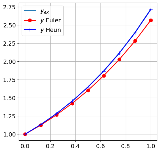
Exercise 13 (Comparing Heun with Euler)
Solve Example 8 with Heun, and plot both the exact solution, \(y_{eul}\) and \(y_{heun}\) for \(N_t = 4, 8, 16, 32\).
# Insert code here.
Solution to Exercise 13 (Comparing Heun with Euler)
t0, T = 0, 1
y0 = 1
lam = 1
Nmax = 8

# rhs of IVP
f = lambda t,y: lam*y

# Compute numerical solution using Euler and Heun
ts, ys_eul = explicit_euler(y0, t0, T, f, Nmax)
ts, ys_heun = heun(y0, t0, T, f, Nmax)

# Exact solution to compare against
y_ex = lambda t: y0*np.exp(lam*(t-t0))
ys_ex = y_ex(ts)

# Plot it
plt.figure()
plt.plot(ts, ys_ex)
plt.plot(ts, ys_eul, 'ro-')
plt.plot(ts, ys_heun, 'b+-')
plt.legend(["$y_{ex}$", "$y$ Euler", "$y$ Heun" ])
<matplotlib.legend.Legend at 0x7f98a1b1df50>
Exercise 14 (Error rates for Heun’s method)
Redo Exercise 12 with Heun.
# Insert code here.
Solution to Exercise 14 (Error rates for Heun's method)
Nmax_list = [4, 8, 16, 32, 64, 128]
error_study(y0, t0, T, f, Nmax_list, heun, y_ex)
For Nmax =   4, max ||y(t_i) - y_i||= 2.343e-02
For Nmax =   8, max ||y(t_i) - y_i||= 6.441e-03
For Nmax =  16, max ||y(t_i) - y_i||= 1.688e-03
For Nmax =  32, max ||y(t_i) - y_i||= 4.322e-04
For Nmax =  64, max ||y(t_i) - y_i||= 1.093e-04
For Nmax = 128, max ||y(t_i) - y_i||= 2.749e-05
The computed error reduction rates are
[3.63726596 3.81482383 3.9067187  3.95322679 3.97658594]
Applying Heun’s and Euler’s method#
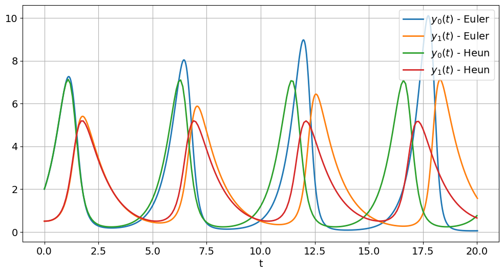
Exercise 15 (The Lotka-Volterra equation revisited)
Solve the Lotka-Volterra equation
In this example, use the parameters and initial values
Use Euler’s method to solve the equation over the interval \([0,20]\), and use \(\tau=0.02\). Try also other step sizes, e.g. \(\tau=0.1\) and \(\tau=0.002\). What do you observe?
Now use Heun’s method with \(\tau=0.1\) Also try smaller step sizes.
Compare Heun’s and Euler’s method. How small do you have to chose the time step in Euler’s method to visually match the solution from Heun’s method?
Note
In this case, the exact solution is not known. What is known is that the solutions are periodic and positive. Is this the case here? Check for different values of \(\tau\).
Solution to Exercise 15 (The Lotka-Volterra equation revisited)
# Reset plotting parameters
plt.rcParams.update({'figure.figsize': (12,6)})

# Define rhs
def lotka_volterra(t, y):
    # Set parameters
    alpha, beta, delta, gamma = 2, 1, 0.5, 1
    # Define rhs of ODE
    dy = np.array([alpha*y[0]-beta*y[0]*y[1],
                   delta*y[0]*y[1]-gamma*y[1]])
    return dy

t0, T = 0, 20            # Integration interval
y0 = np.array([2, 0.5])  # Initital values
# Solve the equation
tau = 0.02
Nmax = int((T-t0)/tau)
print("Nmax = {:4}".format(Nmax))
ts, ys_eul = explicit_euler(y0, t0, T, lotka_volterra, Nmax)

# Plot results
plt.figure()
plt.plot(ts, ys_eul)

# Solve the equation
tau = 0.1
Nmax = int((T-t0)/tau)
print("Nmax = {:4}".format(Nmax))
ts, ys_heun = heun(y0, t0, T, lotka_volterra, Nmax)

plt.plot(ts, ys_heun)
plt.xlabel('t')
plt.legend(['$y_0(t)$ - Euler', '$y_1(t)$ - Euler', '$y_0(t)$ - Heun', '$y_1(t)$ - Heun'],
        loc="upper right" )
Nmax = 1000
Nmax =  200
<matplotlib.legend.Legend at 0x7f989f3d5e90>
Higher order ODEs#
How can we numerically solve higher order ODEs using, e.g., Euler’s or Heun’s method?
Given the \(m\)-th order ODE
For a unique solution, we assume that the initial values
are known.
Such equations can be written as a system of first order ODEs by the following trick: Let
such that
which is nothing but a system of first order ODEs, and can be solved numerically exactly as before.
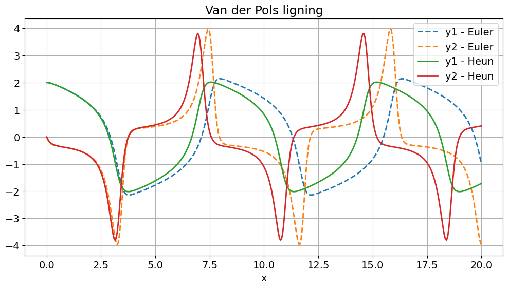
Exercise 16 (Numerical solution of Van der Pol’s equation)
Recalling Example 12, the Van der Pol oscillator is described by the second order differential equation
It can be rewritten as a system of first order ODEs:
a) Let \(\mu=2\), \(u(0)=2\) and \(u'(0)=0\) and solve the equation over the interval \([0,20]\), using the explicit Euler and \(\tau=0.05\). Play with different step sizes, and maybe also with different values of \(\mu\).
b) Repeat the previous numerical experiment with Heun’s method. Try to compare the number of steps you need to perform with Euler vs Heun to obtain visually the “same” solution. (That is, you measure the difference of the two numerical solutions in the “eyeball norm”.)
# Insert code here.
Solution to Exercise 16 (Numerical solution of Van der Pol's equation)
# Define the ODE
def f(t, y):
    mu = 2
    dy = np.array([y[1],
                mu*(1-y[0]**2)*y[1]-y[0] ])
    return dy

# Set initial time, stop time and initial value
t0, T - 0, 20
y0 = np.array([2,0])

# Solve the equation using Euler and plot
tau = 0.05
Nmax = int(20/tau)
print("Nmax = {:4}".format(Nmax))
ts, ys_eul  = explicit_euler(y0, t0, T, f, Nmax)

plt.figure()
plt.plot(ts,ys_eul, "--");

# Solve the equation using Heun
tau = 0.05
Nmax = int(20/tau)
print("Nmax = {:4}".format(Nmax))
ts, ys_heun = heun(y0, t0, T, f, Nmax)

plt.plot(ts,ys_heun);
plt.xlabel('x')
plt.title('Van der Pols ligning')
plt.legend(['y1 - Euler','y2 - Euler', 'y1 - Heun','y2 - Heun'],loc='upper right');
Nmax =  400
Nmax =  400
Observation 6 (Euler vs. Heun)
We clearly see that Heun’s method requires far fewer time steps compared to Euler’s method to obtain the same (visual) solution. For instance, in the case of the Lotka-Volterra example we need with \(\tau \approx 10^{-4}\) roughly 1000x more time steps for Euler than for Heuler’s method, which produced visually the same solution for \(\tau = 0.1\)
Looking back at algorithmic realization of Euler's method and Heun's method we can compare the estimated cost for a single time step. Assuming that the evalution of the rhs \(f\) dominants the overall runtime cost, we observe that Euler’s method requires one function evaluation while Heun’s method’s requires two function evaluation. That means that a single time step in Heun’s method cost roughly twice as much as Euler’s method. With the total number of time steps required by each method, we expect that Heun’s method will result a speed up factor of roughly 500.
Let’s check whether we obtain the estimated speed factor by measuring the executation time of each solution method.
To do so you can use %timeit and %%timeit magic functions in IPython/Jupyterlab,
see corresponding documentation.
In a nutshell, %%timeit measures the executation time of an entire cell, while %timeit
only measures only the executation time of a single line, e.g. as in
%timeit my_function()
Regarding the usage of timeit:
To obtain reliable timeings, timeit does not perform a single run, but
rather a number of runs
%timeit -r <R> -n <N> my_function()
Also if you want to store the value of the best run by passing the option -o:
timings_data = %timeit -o my_function()
which stores the data from the timing experiment. You can access the best time measured in seconds by
timings_data.best
t0, T = 0, 20            # Integration interval
y0 = np.array([2, 0.5])  # Initital values
%%timeit
tau = 1e-4
Nmax = int(20/tau)
ts, ys_eul = explicit_euler(y0, t0, T, lotka_volterra, Nmax)
578 ms ± 2.34 ms per loop (mean ± std. dev. of 7 runs, 1 loop each)
%%timeit
tau = 0.1
Nmax = int(20/tau)
ts, ys_heun = heun(y0, t0, T, lotka_volterra, Nmax)
1.18 ms ± 4.57 μs per loop (mean ± std. dev. of 7 runs, 1,000 loops each)