Numerical solution of ordinary differential equations: Error analysis of one step methods

Numerical solution of ordinary differential equations: Error analysis of one step methods#

As always, we start by importing the necessary modules:

One Step Methods#

In the previous lecture, we introduced the explicit Euler method and Heun’s method. Both methods require only the function \(f\), the step size \(\tau_k\), and the solution \(y_k\) at the current point \(t_k\), without needing information from earlier points \(t_{k-1}, t_{k-2}, \ldots\). This motivates the following definition.

Definition 4 (One step methods)

A one step method (OSM) defines an approximation to the IVP in the form of a discrete function \( {\boldsymbol y}_{\Delta}: \{ t_0, \ldots, t_N \} \to \mathbb{R}^n \) given by

(10)#\[ {\boldsymbol y}_{k+1} := {\boldsymbol y}_k + \tau_k \Phi(t_k, {\boldsymbol y}_{k}, {\boldsymbol y}_{k+1}, \tau_{k}) \]

for some increment function

\[ \Phi: [t_0,T] \times \mathbb{R}^n \times \mathbb{R}^n \times \mathbb{R}^+ \to \mathbb{R}^n. \]

The OSM is called explicit if the increment function \(\Phi\) does not depend on \({\boldsymbol y}_{k+1}\), otherwise it is called implicit.

Example 13 (Increment functions for Euler and Heun)

The increment functions for Euler’s and Heun’s methods are defined as follows:

\[ \Phi(t_k, y_{k}, y_{k+1}, \tau_{k}) = f(t_k, y_k), \qquad \Phi(t_k, y_{k}, y_{k+1}, \tau_{k}) = \tfrac{1}{2} \left( f(t_{k}, y_k) + f\bigl(t_{k+1}, y_{k}+\tau_k f(t_k, y_k) \bigr) \right). \]

Local and global truncation error of OSM#

Definition 5 (Local truncation error)

The local truncation error \(\eta(t, \tau)\) is defined by

(11)#\[ \eta(t, \tau) = y(t) + \tau \Phi(t, y(t), y(t+\tau), \tau) - y(t+\tau). \]

\(\eta(t, \tau)\) is often also called the local discretization or consistency error.

A one step method is called consistent of order \(p\in \mathbb{N}\) if there is a constant \(C > 0\) such that

\[ |\eta(t, \tau) | \leqslant C \tau^{p+1} \quad \text{for } \tau \to 0. \]

A short-hand notation for this is to write \( \eta(t, \tau) = \mathcal{O}(\tau^{p+1})\) for \(\tau \to 0. \)

Example 14 (Consistency order of Euler’s method)

Euler’s method has consistency order \(p=1\).

Definition 6 (Global truncation error)

For a numerical solution \( y_{\Delta}: \{ t_0, \ldots, t_N \} \to \mathbb{R} \) the global truncation error is defined by

(12)#\[ e_k(t_{k-1}, \tau_{k-1}) = y(t_{k}) - y_{k} \quad \text{for } k=1,\ldots,N. \]

A one step method is called convergent with order \(p\in\mathbb{N}\) if

(13)#\[ \max_{k \in \{1,\ldots,N\}} |e_k(t_{k-1},\tau_{k-1})| = \mathcal{O}(\tau^p) \]

with \(\tau = \max_k \tau_k\).

LadyWinderemerFan

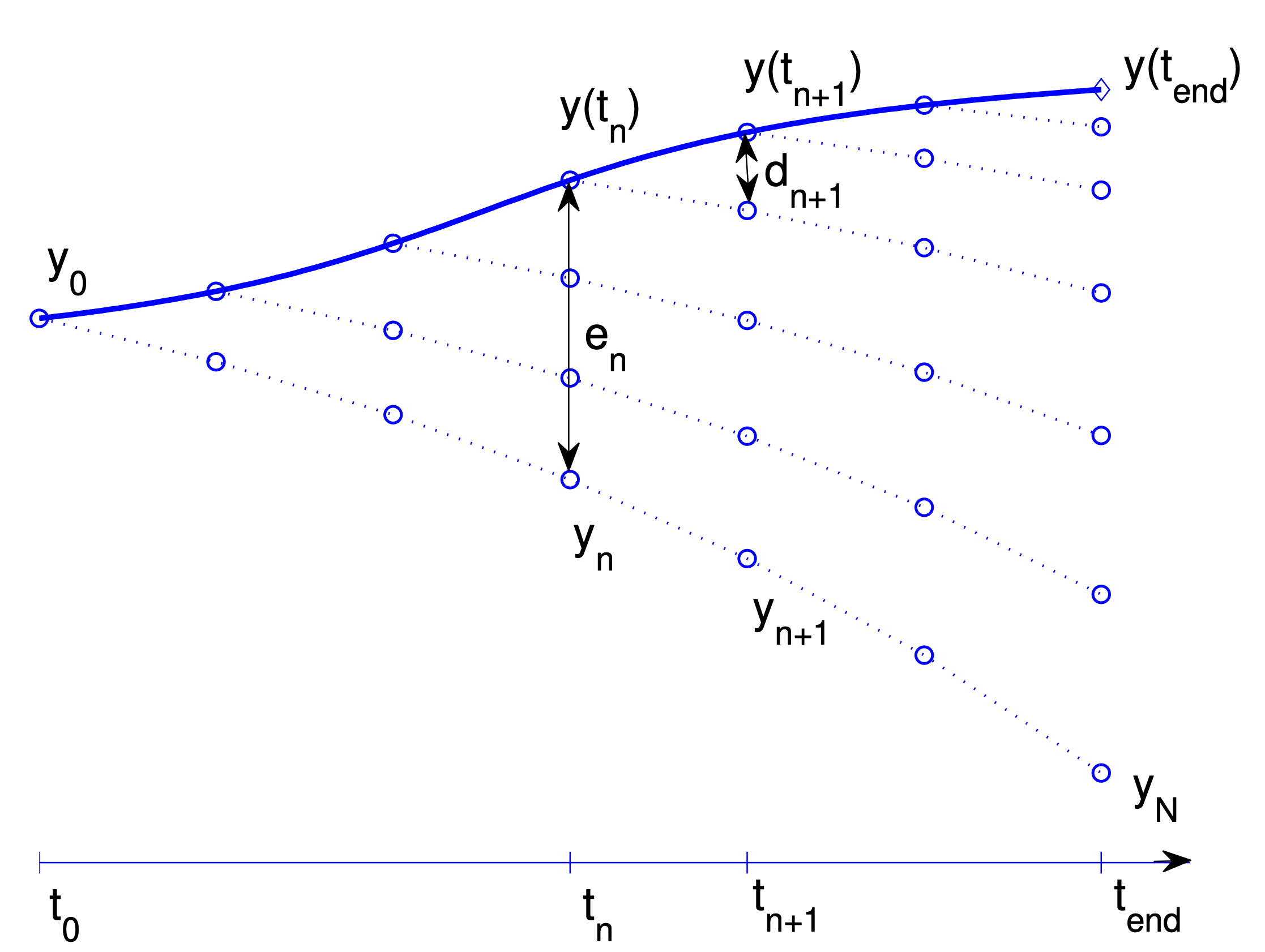
Figure. Lady Windermere’s fan, named after a comedy play by Oscar Wilde. The figure describes the transport and the accumulation of the local truncation errors \(\eta(t_n,\tau_n) =: d_{n+1}\) into the global error \(e_N = y(t_N)-y_N\) at the end point \( t_N = t_{\mathrm{end}}\).

Discussion.

If a one step method has convergence order equal to \(p\), the maximum error \(e(\tau) = \max_k{|e(t_k, \tau)|}\) can be thought as a function of the step size \(\tau\) is of the form

\[ e(\tau) = O(\tau^p) \leqslant C \tau^p. \]

This implies that if we change the time step size from \(\tau\) to e.g. \(\tfrac{\tau}{2}\), we can expect that the error decreases from \(C \tau^p\) to \(C (\tfrac{\tau}{2})^p\), that is, the error will be reduced by a factor \(2^{-p}\).

How can we determine the convergence rate by means of numerical experiments?

Starting from \( e(\tau) = O(\tau^p) \leqslant C \tau^p \) and taking the logarithm gives

\[ \log(e(\tau)) \leqslant p \log(\tau) + \log(C). \]

Thus \(\log(e(\tau))\) is a linear function of \(\log(\tau)\) and the slope of this linear function corresponds to the order of convergence \(p\).

So if you have an exact solution at your disposal, you can for an increasing sequence Nmax_list defining a descreasing sequence of maximum time-steps \(\{\tau_0, \ldots, \tau_N\}\) and solve your problem numerically and then compute the resulting exact error \(e(\tau_i)\) and plot it against \(\tau_i\) in a \(\log-\log\) plot to determine the convergence order.

In addition you can also compute the experimentally observed convergence rate EOC for \(i=1,\ldots M\) defined by

\[ \mathrm{EOC}(i) = \dfrac{ \log(e(\tau_{i})) - \log(e(\tau_{i-1})) }{ \log(\tau_{i}) - \log(\tau_{i-1}) } = \dfrac{ \log(e(\tau_{i})/e(\tau_{i-1})) }{ \log(\tau_{i}/\tau_{i-1}) } \]

Ideally, \(\mathrm{EOC}(i)\) is close to \(p\).

This is implemented in the following compute_eoc function.

def compute_eoc(y0, t0, T, f, Nmax_list, solver, y_ex):
    errs = [ ]
    for Nmax in Nmax_list:
        ts, ys = solver(y0, t0, T, f, Nmax)
        ys_ex = y_ex(ts)
        errs.append(np.abs(ys - ys_ex).max())
        print("For Nmax = {:3}, max ||y(t_i) - y_i||= {:.3e}".format(Nmax,errs[-1]))

    errs = np.array(errs)
    Nmax_list = np.array(Nmax_list)
    dts = (T-t0)/Nmax_list

    eocs = np.log(errs[1:]/errs[:-1])/np.log(dts[1:]/dts[:-1])

    # Insert inf at beginning of eoc such that errs and eoc have same length 
    eocs = np.insert(eocs, 0, np.inf)

    return errs, eocs

Here, solver is any ODE solver wrapped into a Python function which can be called like this

ts, ys = solver(y0, t0, T, f, Nmax)

Exercise 17

Use the compute_eoc function and any of the examples with a known analytical solution from the previous lecture to determine convergence order for Euler’s.

Start from importing the Eulers’s method from the previous lecture,

def explicit_euler(y0, t0, T, f, Nmax):
    ys = [y0]
    ts = [t0]
    dt = (T - t0)/Nmax
    while(ts[-1] < T):
        t, y = ts[-1], ys[-1]  
        ys.append(y + dt*f(t, y))
        ts.append(t + dt)
    return (np.array(ts), np.array(ys))

and copy and complete the following code snippet to compute the EOC for the explicit Euler method:

# Data for the ODE
# Start/stop time
t0, T = ...
# Initial value
y0 = ...
# growth/decay rate
lam = ...

# rhs of IVP
f = lambda t,y: ...

# Exact solution to compare against 
# Use numpy version of exo, namely np.exp 
y_ex = lambda t: ...

# List of Nmax for which you want to run the study
Nmax_list = [... ]

# Run convergence test for the solver
errs, eocs = compute_eoc(...)
print(eocs)

# Plot rates in a table
table = pd.DataFrame({'Error': errs, 'EOC' : eocs})
display(table)
print(table)

# Insert code here.

Solution.

t0, T = 0, 1
y0 = 1
lam = 1

# rhs of IVP
f = lambda t,y: lam*y

# Exact solution to compare against
y_ex = lambda t: y0*np.exp(lam*(t-t0))

Nmax_list = [4, 8, 16, 32, 64, 128, 256, 512]

errs, eocs = compute_eoc(y0, t0, T, f, Nmax_list, explicit_euler, y_ex)
print(eocs)

table = pd.DataFrame({'Error': errs, 'EOC' : eocs})
display(table)
print(table)

For Nmax =   4, max ||y(t_i) - y_i||= 2.769e-01
For Nmax =   8, max ||y(t_i) - y_i||= 1.525e-01
For Nmax =  16, max ||y(t_i) - y_i||= 8.035e-02
For Nmax =  32, max ||y(t_i) - y_i||= 4.129e-02
For Nmax =  64, max ||y(t_i) - y_i||= 2.094e-02
For Nmax = 128, max ||y(t_i) - y_i||= 1.054e-02
For Nmax = 256, max ||y(t_i) - y_i||= 5.290e-03
For Nmax = 512, max ||y(t_i) - y_i||= 2.650e-03
[       inf 0.86045397 0.9243541  0.96050605 0.9798056  0.98978691
 0.99486396 0.99742454]

	Error	EOC
0	0.276876	inf
1	0.152497	0.860454
2	0.080353	0.924354
3	0.041292	0.960506
4	0.020937	0.979806
5	0.010543	0.989787
6	0.005290	0.994864
7	0.002650	0.997425

      Error       EOC
0.276876       inf
0.152497  0.860454
0.080353  0.924354
0.041292  0.960506
0.020937  0.979806
0.010543  0.989787
0.005290  0.994864
0.002650  0.997425

Exercise 18

Redo the previous exercise with Heun’s method.

Start from importing the Heun’s method from yesterday’s lecture.

def heun(y0, t0, T, f, Nmax):
    ys = [y0]
    ts = [t0]
    dt = (T - t0)/Nmax
    while(ts[-1] < T):
        t, y = ts[-1], ys[-1]
        k1 = f(t,y)
        k2 = f(t+dt, y+dt*k1)
        ys.append(y + 0.5*dt*(k1+k2))
        ts.append(t + dt)
    return (np.array(ts), np.array(ys))

# Insert code here.

Solution.

solver = heun
errs, eocs = compute_eoc(y0, t0, T, f, Nmax_list, solver, y_ex)
print(eocs)

table = pd.DataFrame({'Error': errs, 'EOC' : eocs})
display(table)
print(table)

For Nmax =   4, max ||y(t_i) - y_i||= 2.343e-02
For Nmax =   8, max ||y(t_i) - y_i||= 6.441e-03
For Nmax =  16, max ||y(t_i) - y_i||= 1.688e-03
For Nmax =  32, max ||y(t_i) - y_i||= 4.322e-04
For Nmax =  64, max ||y(t_i) - y_i||= 1.093e-04
For Nmax = 128, max ||y(t_i) - y_i||= 2.749e-05
For Nmax = 256, max ||y(t_i) - y_i||= 6.893e-06
For Nmax = 512, max ||y(t_i) - y_i||= 1.726e-06
[       inf 1.86285442 1.93161644 1.96595738 1.98303072 1.99153035
 1.99576918 1.99788562]

	Error	EOC
0	0.023426	inf
1	0.006441	1.862854
2	0.001688	1.931616
3	0.000432	1.965957
4	0.000109	1.983031
5	0.000027	1.991530
6	0.000007	1.995769
7	0.000002	1.997886

      Error       EOC
0.023426       inf
0.006441  1.862854
0.001688  1.931616
0.000432  1.965957
0.000109  1.983031
0.000027  1.991530
0.000007  1.995769
0.000002  1.997886

A general convergence result for one step methods#

Note

In the following discussion, we consider only explicit methods where the increment function \({\boldsymbol \Phi}\) does not depend on \({\boldsymbol y}_{k+1}\).

Theorem 9 (Convergence of one-step methods)

Assume that there exist positive constants \(M\) and \(D\) such that the increment function satisfies

\[ \| {\boldsymbol \Phi}(t,\mathbf{y};\tau) - {\boldsymbol \Phi}(t,\mathbf{z};\tau) \| \leq M \| \mathbf{y}-\mathbf{z} \| \]

and the local trunctation error satisfies

\[ \| {\boldsymbol \eta}(t, \tau) \| = \| \mathbf{y}(t+\tau) - \left (\mathbf{y}(t) + \tau {\boldsymbol \Phi}(t, \mathbf{y}(t), \tau)\right) \| \leqslant D \tau^{p+1} \]

for all \(t\), \(\mathbf{y}\) and \(\mathbf{z}\) in the neighbourhood of the solution.

In that case, the global error satisfies

\[ \max_{k \in \{1,\ldots,N\}} \|e_k(t_{k-1},\tau_{k-1}) \| \leqslant C \tau^p, \qquad C = \frac{e^{M(T-t_0)}-1}{M}D, \]

where \(\tau = \max_{k \in \{0,1,\ldots,N_t\}} \tau_k\).

Proof. We omit the proof here

TODO

Add proof and discuss it in class if time permits.

It can be proved that the first of these conditions are satisfied for all the methods that will be considered here.

Summary.

The convergence theorem for one step methods can be summarized as

“local truncation error behaves like \(\mathcal{O}(\tau^{p+1})\)” + “Increment function satisfies a Lipschitz condition” \(\Rightarrow\) “global truncation error behaves like \(\mathcal{O}(\tau^{p})\)”

or equivalently,

“consistency order \(p\)” + “Lipschitz condition for the Increment function” \(\Rightarrow\) “convergence order \(p\)”.

Convergence properties of Heun’s method#

Thanks to Theorem 9, we need to show two things to prove convergence and find the corresponding convergence of a given one step methods:

determine the local truncation error, expressed as a power series in in the step size \(\tau\)
the condition \(\| {\boldsymbol \Phi}(t,{\boldsymbol y}, \tau) - {\boldsymbol \Phi}(t,{\boldsymbol z},\tau) \| \leqslant M \| {\boldsymbol y} - {\boldsymbol z} \|\)

Determining the consistency order. The local truncation error is found by making Taylor expansions of the exact and the numerical solutions starting from the same point, and compare. In practice, this is not trivial. For simplicity, we will here do this for a scalar equation \(y'(t)=f(t,y(t))\). The result is valid for systems as well

In the following, we will use the notation

\[ f_t = \frac{\partial f}{\partial t}, \qquad f_y = \frac{\partial f}{\partial y}, \qquad f_{tt} = \frac{\partial^2 f}{\partial t^2} \qquad f_{ty} = \frac{\partial^2f}{\partial t\partial y} \qquad\text{etc.} \]

Further, we will surpress the arguments of the function \(f\) and its derivatives. So \(f\) is to be understood as \(f(t,y(t))\) although it is not explicitly written.

The Taylor expansion of the exact solution \(y(t+\tau)\) is given by

\[ y(t+\tau)=y(t)+\tau y'(t) + \frac{\tau^2}{2}y''(t) + \frac{\tau^3}{6}y'''(t) + \dotsm. \]

Higher derivatives of \(y(t)\) can be expressed in terms of the function \(f\) by using the chain rule and the product rule for differentiation.

\[\begin{align*} y'(t) &= f, \\ y''(t) &= f_t + f_y y' = f_t + f_y f,\\ y'''(t) &= f_{tt} + f_{ty} y' + f_{yt}f + f_{yy}y'f + f_yf_t +f_y f_y y' = f_{tt}+2f_{ty}f+f_{yy}f^2 +f_yf_t+ (f_y)^2f. \end{align*}\]

Find the series of the exact and the numerical solution around \(x_0,y_0\) (any other point will do equally well). From the discussion above, the series for the exact solution becomes

\[ y(t_0+\tau) = y_0 + \tau f + \frac{\tau^2}{2}(f_t + f_y f) + \frac{\tau^3}{6}(f_{tt}+2f_{ty}f+f_{yy}f^2 + f_yf_t+ (f_y)^2f ) + \dotsm, \]

where \(f\) and all its derivatives are evaluated in \((t_0,y_0)\).

For the numerical solution we get

\[\begin{align*} k_1 &= f(t_0,y_0) = f, \\ k_2 &= f(t_0+\tau, y_0+\tau k_1) \\ & = f + \tau f_t + f_y\tau k_1 + \frac{1}{2}f_{tt}\tau^2 + f_{ty}\tau \tau k_1 + \frac{1}{2}f_{yy}\tau^2 k_1^2 + \dotsm \\ &= f + \tau(f_t + f_yf) + \frac{\tau^2}{2}(f_{tt} + 2f_{ty}f + f_{yy}f^2) + \dotsm, \\ y_1 &= y_0 + \frac{\tau}{2}(k_1 + k_2) = y_0 + \frac{\tau}{2}(f + f + \tau(f_t + f_yf) + \frac{\tau^2}{2}(f_{tt} + 2f_{ty}k_1 + f_{yy}f^2)) + \dotsm \\ &= y_0 + \tau f + \frac{\tau^2}{2}(f_t+f_yf)+ \frac{\tau^3}{4}(f_{tt} + 2f_{ty}f + f_{yy}f^2) + \dotsm \end{align*}\]

and the local truncation error will be

\[ \eta(t_0, \tau) = y(t_0+\tau)-y_1 = \frac{\tau^3}{12}(-f_{tt}-2f_{ty}f-f_{yy}f^2 + 2f_yf_t + 2(f_y)^2f) + \dotsm \]

The first nonzero term in the local truncation error series is called the principal error term. For \(\tau \) sufficiently small this is the term dominating the error, and this fact will be used later.

Although the series has been developed around the initial point, series around \(x_n,y(t_n)\) will give similar results, and it is possible to conclude that, given sufficient differentiability of \(f\) there is a constant \(D\) such that

\[ \max_i |\eta(t_i, \tau)| \leq D\tau^3. \]

Consequently, Heun’s method is of consistency order \(2\).

Lipschitz condition for \(\Phi\). Further, we have to prove the condition on the increment function \(\Phi(t,y)\). For \(f\) differentiable, there is for all \(y,z\) some \(\xi\) between \(x\) and \(y\) such that \(f(t,y)-f(t,z) = f_y(t,\xi)(y-z)\). Let L be a constant such that \(|f_y|<L\), and for all \(x,y,z\) of interest we get

\[ |f(t,y)-f(t,z)| \leq L |y-z|. \]

The increment function for Heun’s method is given by

\[\begin{split} \Phi(t,y) = \frac{1}{2}(f(t,y)+f(t+\tau,y+\tau f(t,y))). \\ \end{split}\]

By repeated use of the condition above and the triangle inequalitiy for absolute values we get

\[\begin{align*} |\Phi(t,y)-\Phi(t,z)| &= \frac{1}{2}|f(t,y)+f(t+\tau,y+f(t,y))-f(t,z)- f(t+\tau,z+f(t,z)| \\ &\leq \frac{1}{2}\big(|f(t,y)-f(t,z)|+|f(t+\tau,y+\tau f(t,y))-f(t+\tau,z+\tau f(t,z)| \big) \\ &\leq \frac{1}{2}\big(L|y-z| + L|y+\tau f(t,y)-z-\tau f(t,z)| \big) \\ &\leq \frac{1}{2}\big(2L|y-z|+\tau L^2|y-z|\big) \\ & = (L+\frac{\tau}{2}L^2)|y-z|. \end{align*}\]

Assuming that the step size \(\tau\) is bounded upward by some \(\tau_0\), we can conclude that

\[ |\Phi(t,y)-\Phi(t,z)| \leq M|y-z|, \qquad M=L+\frac{\tau_0}{2}L^2. \]

Thanks to Theorem 9, we can conclude that Heun’s method is convergent of order 2.

In the next part, when we introduce a large class of one step methods known as Runge-Kutta methods, of which Euler’s and Heun’s method are particular instances. For Runge-Kutta methods we will learn about some algebraic conditions known as order conditions.