The Discrete Fourier Transform and its applications

Motivation

The discrete Fourier transform and its efficient implementation in form of the so-called Fast Fourier Transform is considered to be among the top 10 most important algorithms in applied mathematics.

In this module we will have its foundation and briefly discuss applications to topics such a signal analysis, image processing/denoising, and the solution of partial differential equations.

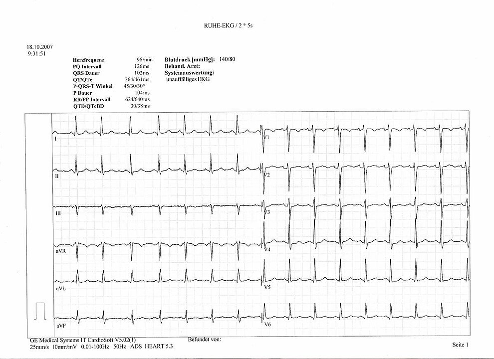Example of an (healthy) electrocardiagraphy.

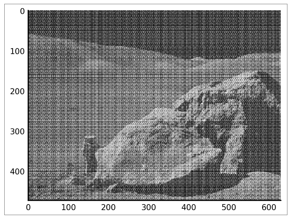Famous noisy image of the moon landing.

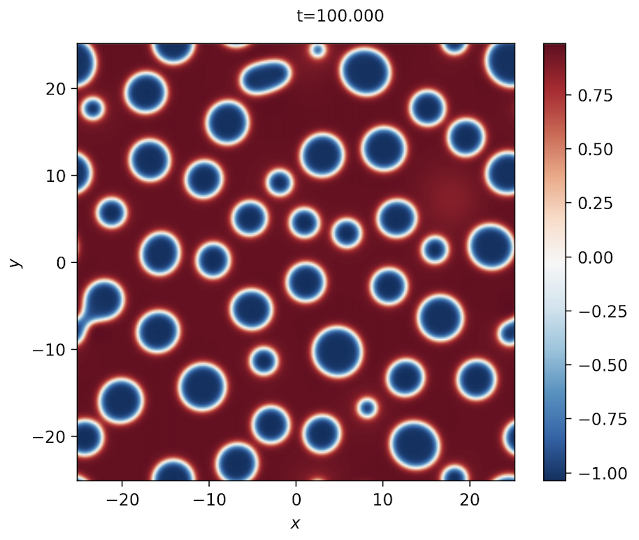Snapshot of the Cahn-Hilliard equation modeling phase separation.

Preliminaries

First we recall some fundamental concepts, ideas and identities from Matte 4K, see in particular week 35 - week 38.

Complex numbers

[Complex numbers]

\(z = a + bi\) where \(a\) and \(b\) are real numbers and \(i = \sqrt{-1}\) is the imaginary unit. We write \(\Re(z) = a\) and \(\Im(z) = b\) for the real and imaginary part of \(z\).

[Complex conjugate]

of \(z\) is \(\bar{z} = a - bi\).

[Euler’s formula]

\(e^{i\theta} = \cos \theta + i\sin\theta\).

[Polar form]

\(z = x + iy = r e^{i\theta}\) where \(r = |z| = \sqrt{x^2+y^2}\) is the magnitude and \(\theta = \arg z = \arctan(y/x)\) is the argument or phase.

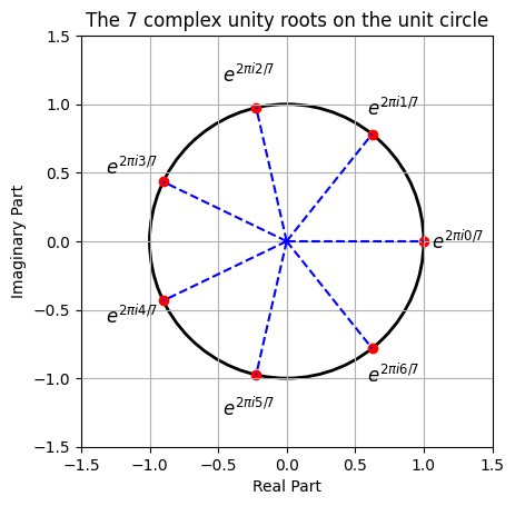
[n-th roots of unity]

For given \(n\), the \(N\)-th roots of unity are the solutions to the equation \(z^n = 1\). There are \(n\) distinct roots which are given by

\[ \omega_N^k = e^{2\pi i k/N} \quad \text{for } k = 0, 1, \ldots, N-1. \]

(four:eq:unityroots)

Observation 8

We have the following easily verifiable properties of the roots of unity for \(k,l \in \mathbb{Z}\):

\[ (\omega_N^{k})^l = \omega_N^{lk} = (\omega_N^l)^k, \qquad \omega_N^{k+l} = \omega_N^k\omega_N^l, \qquad \overline{\omega_N^k} = \omega_N^{-k}, \qquad \omega_N^{k+N} = \omega_N^k. \]

Show code cell source Hide code cell source

import matplotlib.pyplot as plt
import numpy as np

def plot_complex_unity_roots(n):
    # Calculate the roots
    roots = [np.exp(2j * np.pi * k / n) for k in range(n)]
    
    # Extract real and imaginary parts
    real_parts = [root.real for root in roots]
    imag_parts = [root.imag for root in roots]
    
    # Plot the unit circle
    circle = plt.Circle((0, 0), 1, color='black', fill=False, linestyle='-', linewidth=2)
    
    fig, ax = plt.subplots()
    ax.add_artist(circle)
    
    # Plot the roots
    ax.scatter(real_parts, imag_parts, color='red')
    
    # Add grid
    ax.grid(True)
    
    # Add labels to the roots
    for k, (real, imag) in enumerate(zip(real_parts, imag_parts)):
        # Draw a line from the origin to the root
        ax.plot([0, real], [0, imag], color='blue', linestyle='--')
        label = f'$e^{{2\\pi i {k}/{n}}}$'
        # Move the label just outside the circle
        ax.text(real * 1.25, imag * 1.25, label, fontsize=12, ha='center', va='center')
    
    # Set equal aspect ratio
    ax.set_aspect('equal')
    
    # Set limits
    ax.set_xlim(-1.5, 1.5)
    ax.set_ylim(-1.5, 1.5)
    
    # Add labels
    ax.set_xlabel('Real Part')
    ax.set_ylabel('Imaginary Part')
    ax.set_title(f'The {n} complex unity roots on the unit circle')
    
    plt.show()

# Example usage
plot_complex_unity_roots(7)

# TODO: Present operation of complex numbers in Python
z1 = complex(1,2)
print(z1)
z2 = 1 + 2j
print(z2)

(1+2j)
(1+2j)

Complex inner product spaces and orthogonal systems

Definition 10 (Complex inner product space)

Let \(V\) be a complex vector space. An inner product on \(V\) is a function \(\langle \cdot, \cdot \rangle : V \times V \to \mathbb{C}\) that satisfies the following properties for all \(f,g,h \in V\) and all \(\alpha,\beta \in \mathbb{C}\):

1. Linearity in the first argument:

   \[ \langle \alpha f + \beta g, h \rangle = \alpha \langle f,h \rangle + \beta \langle g,h \rangle. \]

2. Conjugate symmetry:

   \[ \langle f,g \rangle = \overline{\langle g,f \rangle}. \]

3. Positive definiteness:

   \[ \langle f,f \rangle \geq 0, \]
   with equality if and only if \(f = 0\).

As with all inner product spaces, a norm by

(29)\[ \|f\| = \sqrt{\langle f,f \rangle}. \]

and we have the Cauchy-Schwarz inequality

(30)\[ |\langle f,g \rangle| \leqslant \|f\| \|g\|. \]

For an inner product space, the Cauchy-Schwarz inequality holds

\[ |\langle f,g \rangle| \leqslant \|f\| \|g\| \]

and equality holds if and only if \(f\) and \(g\) are linearly dependent.

Definition 11 (Orthogonal system)

A sequences/family \(\{\phi_n\}_{n\in \mathbb{N}}\) of non-zero vectors \(\phi_n\) in a complex inner product space \(V\) is said to be orthogonal if

\[ \langle \phi_n, \phi_m \rangle = 0, \quad n \neq m. \]

If in addition \(\|\phi_n\| = 1\) for all \(n\), then the system is said to be orthonormal.

For a given interval \([a,b]\), we define the set of square-integrable, possibly complex-valued function \(L^2(I)\) by

(31)\[ L^2(I) = \left\{ f: I \to \mathbb{C} \mid \int_I |f(x)|^2 dx < \infty \right\}. \]

Here, the interval \(I\) can be either finite, semi-infinite or infinite, i.e., the end point choices \(a = -\infty\) and/or \(b=\infty\) are allowed.

For \(f,g \in L^2(I)\), an inner product is defined by

(32)\[ \langle f,g \rangle = \int_I f(x) \bar{g}(x) dx. \]

From hereon, we think of \(L^2(I)\) as a inner product space equipped with the inner product defined by (32).

Set \([a,b] = [-\pi, \pi]\). We have the following orthogonal systems in \(L^2([-\pi,\pi])\).

Example 16

The set of functions \(\{e^{inx}\}_{n \in \mathbb{Z}}\) is an orthogonal system in \(L^2([-\pi,\pi])\). Correspondingly, the set \(\{e^{inx}/\sqrt{2\pi}\}_{n \in \mathbb{Z}}\) is an orthonormal system in \(L^2([-\pi,\pi])\).

The set of functions

\[ \{e^{inx}\}_{n \in \mathbb{Z}} \quad \text{and} \quad \{e^{inx}/\sqrt{2\pi}\}_{n \in \mathbb{Z}} \]

are orthogonal and orthonormal system in \(L^2([-\pi,\pi])\), respectively.

Example 17

The set of functions

\[ \{1\} \cup \{\cos(nx)\}_{n=1}^\infty \cup \{\sin(nx)\}_{n=1}^\infty \quad \text{and} \quad \{1/\sqrt{2\pi}\} \cup \{\cos(nx)/\sqrt{\pi}\}_{n=1}^\infty \cup \{\sin(nx)/\sqrt{\pi}\}_{n=1}^\infty \]

are orthogonal and orthonormal systems in \(L^2([-\pi,\pi])\), respectively.

Fouries series

Let’s consider a periodic function \(f(x)\) with period \(2\pi\), i.e., \(f(x+2\pi) = f(x)\) for all \(x\). Then the formal complex Fourier series of \(f(x)\) is given by

(33)\[ f(x) = \sum_{k=-\infty}^{\infty} c_k e^{i k x} \]

where \(\{c_k\}_{k\in\mathbb{Z}}\) are the Fourier coefficients given by

(34)\[ c_k = \frac{1}{2\pi} \int_{-\pi}^{\pi} f(x) e^{-i k x} \, d\mathrm{x} \]

We denote by \(S_N(f,x)\) the \(N\)-th partial sum of the Fourier series of \(f(x)\), i.e.,

(35)\[ S_N(f,x) = \sum_{k=-N}^{N} c_k e^{i k x}. \]

We recall that \(S_N(f,x)\) can we rewritten in terms of \(\sin\) and \(\cos\) functions:

(36)\[ \sum_{k=-n}^{n} c_k e^{i k x} = \dfrac{a_0}{2} + \sum_{k=1}^{N} a_k \cos(kx) + b_k \sin(kx), \]

where

\[ a_0 = 2 c_0, \quad a_k = c_k + c_{-k}, \quad b_k = i(c_k - c_{-k}). \]

We set \(L^2_p([-\pi,\pi])\) to be the set of periodic functions with period \(2\pi\) which are square-integrable over some (and thus any) interval \([a, a+2\pi]\) of length \(2\pi\).