Exercises on the discrete Fourier transform

Exercise 28

Consider two periodic functions \(f(x)\) and \(g(x)\) with period \(L=2\) and their truncated Fourier series \(f_N(x)\) and \(g_N(x)\). The errors \(E_N\) between each function and its trigonometric approximation can be computed using Parseval’s identity,

\[\begin{align*} E_N = \int_{-1}^{1} f^2(x)\,\mathrm{d}x - 2 \sum_{k=-N}^N |c_k|^2\, . \end{align*}\]

a) Let \(f(x) = \mathrm{e}^{-x}\) for \(x \in [-1,1)\) and consider its periodic extension with period \(L=2\). Find on the Fourier coefficients of \(f(x)\), calculate the error \(E_N\) for \(N=2\), \(4\) and \(8\).

b) Now, do the same for \(g(x) = \mathrm{e}^{-|x|}\).

c) Why is the error so much larger when approximating \(f(x)\) than in the case of \(g(x)\)?

Solution to Exercise 28

a) We first find the Fourier coefficients,

(77)\[\begin{align} c_k = \frac{1}{2}\int_{-1}^{1} e^{-(1 + i k \pi) x} \, dx = \frac{(-1)^k \sinh(1)}{1+ik\pi}, \end{align}\]

and then integrate

\[\begin{align*} \int_{-1}^{1} f^2(x)\mathrm{d}x = \int_{-1}^{1} e^{-2x} \mathrm{d}x = \frac{e^{2}-e^{-2}}{2} = \sinh(2), \end{align*}\]

Then we get an expression for the error,

\[\begin{align*} E_N = \sinh(2) - 2 \sum_{k=-N}^N \frac{\sinh^2(1)}{(1+ik\pi)^2} = \sinh(2) - \sum_{k=-N}^N \frac{2\sinh^2(1)}{1+k^2\pi^2}. \end{align*}\]

Inserting values for N: \(E_2=0.22, E_4=0.123, E_8=0.066\)

b) Now, we find the Fourier coefficients for \(g(x)\)

\[\begin{align*} c_k &= \frac{1}{2}\int_{-1}^{1}\mathrm{e}^{-|x|}\mathrm{e}^{-ik\pi x}\, \mathrm{d}x = \frac{1}{1+k^2\pi^2} \left( 1 - \mathrm{e}^{-1} (-1)^k \right). \end{align*}\]

As in a), we need to compute the integral of g(x) squared

\[\begin{align*} \int_{-1}^{1} g^2(x)\mathrm{d}x = \int_{-1}^{1} e^{-2|x|} \mathrm{d}x = 1-e^{-2}, \end{align*}\]

\[\begin{align*} E_N = 1-e^{-2} - 2\sum_{k=-N}^N \left( \frac{1}{1+k^2\pi^2} \left( 1 - \mathrm{e}^{-1} (-1)^k \right) \right)^2. \end{align*}\]

Inserting values for N gives: \(E_2=1.19e-3, E_4=2e-4, E_8=2.8e-5\)

c) \(g(x)\) is smoother than \(f(x)\) and the Fourier series for \(g(x)\) are therefor a better approximation.

Exercise 29

a) Use DFT (by hand) to find the coefficients \(c_k\) for the trigonometric polynomial which interpolates the following datapoints

t	0	0.25	0.5	0.75
Datapoint	1+i	i	-1-i	-i

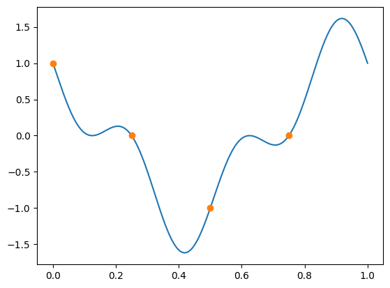
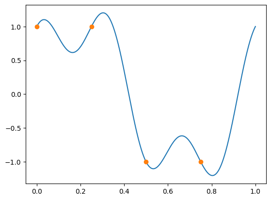
b) Plot (using Python) the real and imaginary parts of corresponding interpolation polynomial \(Q_k(t) = \frac{1}{n} \sum^{n-1}_{k=0} c_k e^{2\pi i k t} \), together with the datapoints.

Solution to Exercise 29

We have four datapoints, and recall the definition of \( \omega_N^{-1} = e^{-2\pi i / n} = e^{-i\pi/2} = -i \), use this in the Fourier matrix,

(78)\[\begin{align} F_4 = \dfrac{1}{4} \begin{pmatrix} 1 & 1 & 1 & 1 \\ 1 & \omega_N^{-1} & \omega_N^{-2} & \omega_N^{-3} \\ 1 & \omega_N^{-2} & \omega_N^{-4} & \omega_N^{-6} \\ 1 & \omega_N^{-3} & \omega_N^{-6} & \omega_N^{-9} \\ \end{pmatrix} = \dfrac{1}{4} \begin{pmatrix} 1 & 1 & 1 & 1 \\ 1 & -i & -1 & i \\ 1 & -1 & 1 & -1 \\ 1 & i & -1 & -i \\ \end{pmatrix} \end{align}\]

We can then multiply the matrix with the vector of datapoints and get the coefficients,

(79)\[\begin{align} c_k = \dfrac{1}{4} F_4 D_4 = \dfrac{1}{4}[0 , 4 + 2i, 0, 2i]. \end{align}\]

import numpy as np
import matplotlib.pyplot as plt

N = 4 
datapoints = np.array([1+1j,1j,-1-1j,-1j])
t = np.array([0,0.25,0.5,0.75])
c_k = 1/N*np.array([0,4 + 2j,0,2j]) #found by matrix multiplication as above

x = np.linspace(0,1,10000)

#build the interpolation polynomial
S_N = c_k[0]
for i in range(1,N):
    S_N += c_k[i]*np.exp(2j*np.pi*x*i)
    

plt.plot(x, S_N.real)
plt.plot(t, datapoints.real,marker='o', linestyle='')
plt.show()

plt.plot(x, S_N.imag)
plt.plot(t, datapoints.imag,marker='o', linestyle='')
plt.show()

Exercise 30

In this task we use the datapoints given in the codeblock below

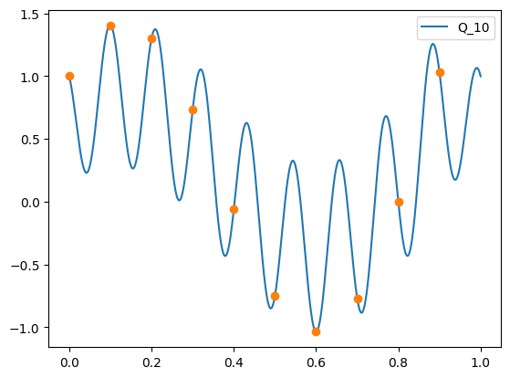
a) Interpolate using DFT, this time using numpy/scipy to find the coefficients. Plot the corresponding trigonometric interpolation polynomial \(Q_{10}\), and check that it interpolates the datapoints.

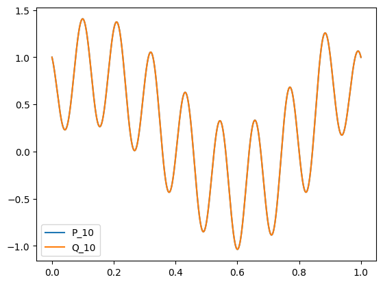
b) Using the Euler formula, and fact that all datapoints are real-valued, we have the following formula to rewrite \(Q_{10}\),

\[\begin{align*} P_n(t) = \frac{1}{n} \sum^{n-1}_{k=0} a_k \cos(2\pi i k t) - b_k \sin(2\pi i k t), \end{align*}\]

where \( c_k = a_k + i b_k\). Plot \(P_{10}\) and check that it is the same as \(Q_{10}\).

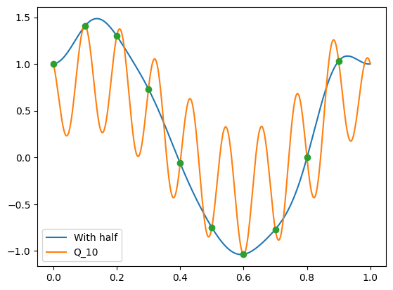
c) Try plotting

\[\begin{align*} \tilde{P}_{10} = \frac{a_0}{n} + \frac{2}{n} \sum^{n/2-1}_{k=0} (a_k \cos(2\pi i k t) - b_k \sin(2\pi i k t)) + \frac{a_{n/2}}{n}\cos(\pi i t) \end{align*} \]

Explain why \(\tilde{P}_{10}\) also interpolates the same datapoints, with only half of the Fourier terms

Solution to Exercise 30

datapoints=np.array([ 1.0, 1.40680225, 1.30007351, 0.73203952, -0.06123174, -0.75, -1.03680225, -0.77007351, -0.00203952, 1.03123174])
t = np.array([0. , 0.1, 0.2, 0.3, 0.4, 0.5, 0.6, 0.7, 0.8, 0.9])

N = 10
x = np.linspace(0,1,10000)  
dft = np.fft.fft(datapoints)

Q_N = dft[0]*1/N
for i in range(1,N):
    Q_N += 1/(N)*dft[i]*np.exp(2j*np.pi*x*i)
    

plt.plot(x, Q_N.real,label="Q_10")
plt.plot(t, datapoints,marker='o', linestyle='')
plt.legend()
plt.show()

P_N = dft[0].real*1/N#*np.exp(x*1j*0)
for i in range(1,N):
    P_N += 1/(N)*(dft[i].real*np.cos(i*2*np.pi*x) - dft[i].imag*np.sin(i*2*np.pi*x))
    

plt.plot(x, P_N.real, label='P_10')
plt.plot(x, Q_N.real,label="Q_10")
plt.legend()
plt.show()

P_N2 = dft[0].real*1/N#*np.exp(x*1j*0)
for i in range(1,int(N/2)):
    P_N2+= 2/(N)*(dft[i].real*np.cos(i*2*np.pi*x) - dft[i].imag*np.sin(i*2*np.pi*x))
P_N2 += 1/(N)*dft[int(N/2)].real*np.cos(N*np.pi*x)

plt.plot(x, P_N2.real, label='With half')
plt.plot(x, Q_N.real,label="Q_10")
plt.plot(t, datapoints,marker='o', linestyle='')
#plt.plot(x, func(x).real)
plt.legend()
plt.show()

If we have real-valued datapoints \(x_k\), and do a DFT to get \(c_k\), we have that \(c_0\) is real valued, and \(c_{n-k} = \bar{c}_k\) (you can print out the dft above and check). Using also the trigonometric identities \(\cos(2(n-k)\pi t) = \cos(2k\pi t), \sin(2(n-k)\pi t) = -\sin(2k\pi t) \), we will get the formula above (for an even number datapoints, a similar exists of odd number of datapoints).