Numerical solution of ordinary differential equations: Stiff problems

Numerical solution of ordinary differential equations: Stiff problems#

And of course we want to import the required modules.

# import matplotlib.font_manager
# matplotlib.font_manager.findfont("Humor Sans")

Explicit Euler method and a stiff problem#

We start by taking a second look at the IVP

(21)#\[ y'(t) = \lambda y(t), \quad y(t_0) = y_0. \]

with the analytical solution

(22)#\[\begin{equation} y(t) = y_0 e^{\lambda(t-t_0)}. \end{equation}\]

Recall that for \(\lambda > 0\) this equation can present a simple model for the growth of some population, while a negative \(\lambda < 0\) typically appears in decaying processes (read “negative growth”).

So far we have only solved ((21)) numerically for \(\lambda > 0\). Let’s start with a little experiment. First, we set \(y_0 = 1\) and \(t_0 = 0\). Next, we chose different \(\lambda\) to model processes with various decay rates, let’s say

\[ \lambda \in \{ -10, -50, -250\}. \]

For each of those \(\lambda\), we set a reference step length

\[ \tau_{\lambda} = \dfrac{2}{|\lambda|} \]

(we will soon see why!) and compute a numerical solution using the explict Euler method for three different time steps, namely for \( \tau \in \{ 0.1 \tau_{\lambda}, \tau_{\lambda}, 1.1 \tau_{\lambda} \} \) and plot the numerical solution together with the exact solution.

def explicit_euler(y0, t0, T, f, Nmax):
    ys = [y0]
    ts = [t0]
    dt = (T - t0)/Nmax
    while(ts[-1] < T):
        t, y = ts[-1], ys[-1]  
        ys.append(y + dt*f(t, y))
        ts.append(t + dt)
    return (np.array(ts), np.array(ys))

plt.rcParams['figure.figsize'] = (16.0, 12.0)
t0, T = 0, 1
y0 = 1
lams = [-10, -50, -250]

fig, axes = plt.subplots(3,3)
fig.tight_layout(pad=3.0)

for i in range(len(lams)):
    lam = lams[i]
    tau_l = 2/abs(lam)
    taus = [0.1*tau_l, tau_l, 1.1*tau_l]

    # rhs of IVP
    f = lambda t,y: lam*y

    # Exact solution to compare against
    y_ex = lambda t: y0*np.exp(lam*(t-t0))

    # Compute solution for different time step size
    for j in range(len(taus)):
        tau = taus[j]
        Nmax = int(1/tau)
        ts, ys = explicit_euler(y0, t0, T, f, Nmax)
        ys_ex = y_ex(ts)
        axes[i,j].set_title(f"$\\lambda = {lam}$, $\\tau = {tau:0.2f}$")
        axes[i,j].plot(ts, ys, "ro-")
        axes[i,j].plot(ts, ys_ex)
        axes[i,j].legend([r"$y_{\mathrm{FE}}$", "$y_{\\mathrm{ex}}$"])

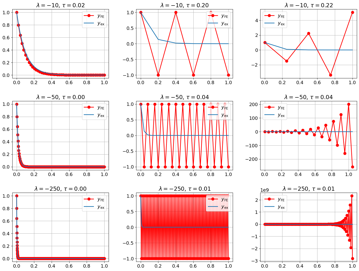
../_images/86aa2288805261beacc080320b262e82b33d086007ce877ffceac22969a45496.png

Observation 7

Looking at the first column of the plot, we observe a couple of things. First, the numerical solutions computed with a time step \(\tau = 0.1 \tau_{\lambda}\) closely resembles the exact solution. Second, the exact solution approaches for larger \(t\) a stationary solution (namely 0), which does not change significantly over time. Third, as expected, the exact solution decays the faster the larger the absolute value of \(\lambda\) is. In particular for \(\lambda = -250\), the exact solution \(y_{\mathrm{ex}}\) drops from \(y_{\mathrm{ex}}(0) = 1\) to \(y_{\mathrm{ex}}(0.05) \approx 3.7\cdot 10^{-6}\) at \(t = 0.05\), and at \(t=0.13\), the exact solution is practically indistinguishable from \(0\) as \(y_{\mathrm{ex}}(0.13) \approx 7.7\cdot 10^{-16}\).

Looking at the second column, we observe that a time-step size \(\tau = \tau_{\lambda}\), the numerical solution oscillates between \(-1\) and \(1\), and thus the numerical solution does not resemble at all the monotonic and rapid decrease of the exact solution. The situation gets even worse for a time-step size \(\tau > \tau_{\lambda}\) (third column) where the the numerical solution growths exponentially (in absolute values) instead of decaying exponentially as the \(y_{\mathrm{ex}}\) does.

So what is happening here? Why is the explicit Euler method behaving so strangely? Having a closer look at the computation of a single step in Euler’s method for this particular test problem, we see that

\[\begin{align*} y_{i+1} &= y_i + \tau f(t_i, y_i) = y_i + \tau \lambda y_i = (1 + \tau \lambda) y_i = (1 + \tau \lambda)^2 y_{i-1} = \ldots = (1 + \tau \lambda)^{i+1} y_0 \end{align*}\]

Thus, for this particular IVP, the next step \(y_{i+1}\) is simply computed by by multiplying the current value \(y_i\) with the the function \((1+\tau\lambda)\).

\[\begin{align*} y_{i+1} = R(z)^{i+1} y_0, \quad z = \tau \lambda \end{align*}\]

where \(R(z) = (1+z)\) is called the stability function of the explicit Euler method.

Now we can understand what is happening. Since \(\lambda < 0\) and \(\tau > 0\), we see that as long as \( \tau \lambda > - 2 \Leftrightarrow \tau < \dfrac{2}{|\lambda|} \), we have that \(|1 + \tau \lambda| < 1\) and therefore, \(|y_i| = |1 + \tau \lambda|^{i+1} y_0\) is decreasing and converging to \(0\) For \(\tau = \dfrac{2}{|\lambda|} = \tau_{\lambda}\), we obtain

\[ y_{i+1} = (1 + \tau \lambda)^{i+1} y_0 = (-1)^{i+1} y_0 \]

so the numerical solution will be jump between \(-1\) and \(1\), exactly as observed in the numerical experiment. Finally, for \(\tau > \dfrac{2}{|\lambda|} = \tau_{\lambda}\), \(|1 + \tau \lambda| > 1\), and \(|y_{i+1}| = |1 + \tau \lambda|^{i+1} y_0\) is growing exponentially.

Note, that is line of thoughts hold independent of the initial value \(y_0\). So even if we just want to solve our test problem ((21)) away from the transition zone where \(y_{\mathrm{ex}}\) drops from \(1\) to almost \(0\), we need to apply a time-step \(\tau < \tau_{\lambda}\) to avoid that Euler’s method produces a completely wrong solution which exhibits exponential growth instead of exponential decay.

Summary

For the IVP problem stiff:ode:eq:exponential, Euler’s method has to obey a time step restriction \(\tau < \dfrac{2}{|\lambda|}\) to avoid numerical instabilities in the form of exponential growth.

This time restriction becomes more severe the larger the absolute value of \(\lambda < 0\) is. On the other hand, the larger the absolute value of \(\lambda < 0\) is, the faster the actual solution approaches the stationary solution \(0\). Thus it would be reseaonable to use large time-steps when the solution is close to the stationary solution. Nevertheless, because of the time-step restriction and stability issues, we are forced to use very small time-steps, despite the fact that the exact solution is not changing very much. This is a typical characteristic of a stiff problem. So the IVP problem stiff:ode:eq:exponential gets “stiffer” the larger the absolute value of \(\lambda < 0\) is, resulting in a severe time step restriction \(\tau < \dfrac{2}{|\lambda|}\) to avoid numerical instabilities.

Outlook. Next, we will consider other one-step methods and investigate how they behave when applied to the test problem stiff:ode:eq:exponential. All these one step methods will have a common, that the advancement from \(y_{k}\) to \(y_{k+1}\) can be written as

\[ y_{k+1} = R(z) y_{k} \quad \text{with } z = \tau \lambda \]

for some stability function \(R(z)\).

With our previous analysis in mind we will introduce the following

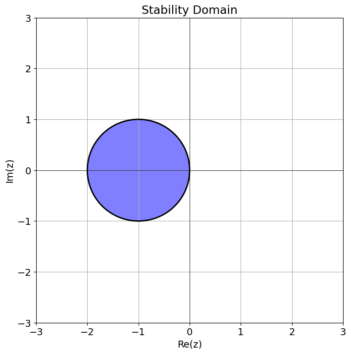
Definition 9 (Stability domain)

Let \(R(z)\) be the stability function for some one-step function. Then the domain

(23)#\[ \mathcal{S} = \{ z \in \mathbb{R}: |R(z)| \leqslant 1 \} \]

is called the domain of stability.

Remark 4

Usually, one consider the entire complex plane in the definition of the domain of stability, that is, \(\mathcal{S} = \{ z \in \mathbb{C}: |R(z)| \leqslant 1 \}\) but in this course we can restrict ourselves to only insert real arguments in the stability function.

Let’s plot the domain of stability for the explicit Euler method.

def r_fe(z):
    return 1 + z

plot_stability_domain(r_fe)

../_images/c06142ee509a7b65363fe9c30e585bfa3301d841bba548bfc0d7651951d405a8.png

Important

Time-step restrictions for explicit RKM

Unfortunately, all explicit Runge-Kutta methods when applied to the simple test problem (21) will suffer from similar problems as the explicit Euler method, for the following reason:

It can be shown that for any explicit RKM, its corresponding stability function \(r(z)\) must be a polynomial in \(z\). Since complex polynomials satisfy \(|r(z)| \to \infty\) for \(|z| \to \infty\), its domain of stability as defined above must be bounded. Consequently, there will a constant \(C\) such that any time step \(\tau > \dfrac{C}{|\lambda|}\) will lead to numerical instabilities.

The implicit Euler method#

Previously, we considered Euler’s method, for the first-order IVP

\[ y'(t) = f(t,y(t)), \qquad y(t_0)=y_0 \]

where the new approximation \(y_{k+1}\) at \(t_{k+1}\) is defined by

\[ y_{k+1} := y_{k} + \tau f(t_{k}, y_{k}) \]

We saw that this could be interpreted as replacing the differential quotient \(y'\) by a forward difference quotient

\[ f(t_k,y_k) = y'(t_k) \approx \dfrac{y(t_{k+1}) - y(t_k)}{\tau} \]

Here the term “forward” refers to the fact that we use a forward value \(y(t_{k+1})\) at \(t_{k+1}\) to approximate the differential quotient at \(t_k\).

Now we consider a variant of Euler’s method, known as the implicit or backward Euler method. This time, we simply replace the differential quotient \(y'\) by a backward difference quotient

\[ f(t_k,y_k) = y'(t_k) \approx \dfrac{y(t_{k}) - y(t_{k-1})}{\tau} \]

resulting in the following

Algorithm 3 (Implicit/backward Euler method)

Given a function \(f(t,y)\) and an initial value \((t_0,y_0)\).

Set \(t = t_0\), choose \(\tau\).
\(\texttt{while } t < T\):
- \(\displaystyle y_{k+1} := y_{k} + \tau f(t_{k+1}, y_{k+1})\)
- \(t_{k+1}:=t_k+\tau\)
- \(t := t_{k+1}\)

Note that in contrast to the explicit/forward Euler, the new value of \(y_{k+1}\) is only implicitly defined as it appears both on the left-hand side and right-hand side. Generally, if \(f\) is nonlinear in its \(y\) argument, this amounts to solve a non-linear equation, e.g., by using fix-point iterations or Newton’s method. But if \(f\) is linear in \(y\), that we only need to solve a linear system.

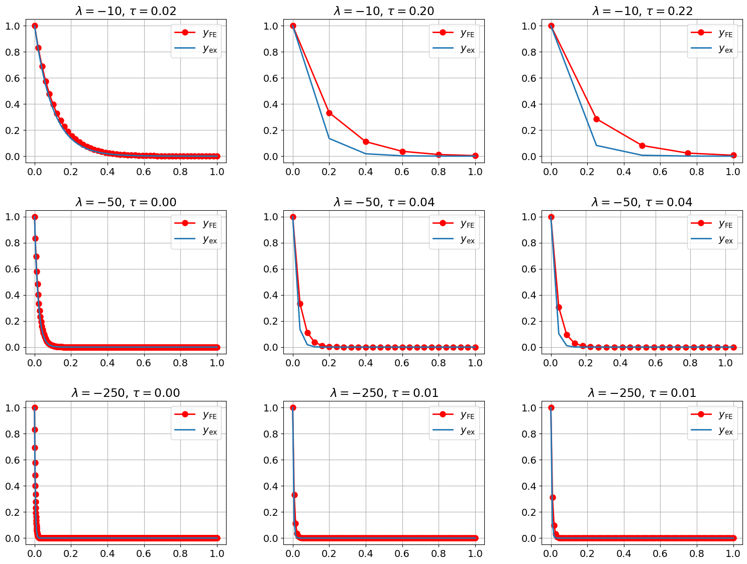
Let’s see what we get if we apply the backward Euler method to our model problem.

Exercise 25 (Implicit/backward Euler method)

a) Show that the backward difference operator (and therefore the backward Euler method) has consistency order \(1\), that is,

\[ y(t) + \tau f(t+\tau, y(t+\tau)) - y(t+\tau) = \mathcal{O}(\tau^2) \]

b) Implement the implicit/backward Euler method

        def implicit_euler(y0, t0, T, lam, Nmax):
          ...

for the IVP ((21)). Note that we now take \(\lambda\) as a parameter, and not a general function \(f\) as we want to keep as simple as possible Otherwise we need to implement a nonlinear solver if we allow for arbitrary right-hand sides \(f\). You use the code for explicit_euler as a start point.

c) Write down the Butcher table for the implicit Euler method.

d) Rerun the numerical experiment from the previous section with the implicit Euler method. Do you observe any instabilities?

e) Find the stability function \(R(z)\) for the implicit Euler satisfying

(24)#\[\begin{equation} y_{k+1} = R(\tau \lambda) y_{k} \end{equation}\]

and use it to explain the much better behavior of the implicit Euler when solving the initial value problem (21).

Solution to Exercise 25 (Implicit/backward Euler method)

a) As before, we simply do a Taylor expansion of \(y\), but this time around \(t+\tau\). Then

\[ y(t) = y(t+ \tau) - \tau y'(t+ \tau) + \mathcal{O}(\tau^2) = y(t+ \tau) - \tau f(t+ \tau, y(t+ \tau)) + \mathcal{O}(\tau^2) \]

which after rearranging terms is exactly (4).

b)

# Warning, implicit Euler is only implement for the test equation
# not a general f!
def implicit_euler(y0, t0, T, lam, Nmax):
    ys = [y0]
    ts = [t0]
    dt = (T - t0)/Nmax
    while(ts[-1] < T):
        t, y = ts[-1], ys[-1]  
        ys.append(y/(1-dt*lam))
        ts.append(t + dt)
    return (np.array(ts), np.array(ys))

c)

\[\begin{split} \begin{array}{c|c} 1 & 1 \\ \hline & 1 \end{array} \end{split}\]

d)

plt.rcParams['figure.figsize'] = (16.0, 12.0)
t0, T = 0, 1
y0 = 1
lams = [-10, -50, -250]

fig, axes = plt.subplots(3,3)
fig.tight_layout(pad=3.0)

for i in range(len(lams)):
    lam = lams[i]
    tau_l = 2/abs(lam)
    taus = [0.1*tau_l, tau_l, 1.1*tau_l]

    # rhs of IVP
    f = lambda t,y: lam*y

    # Exact solution to compare against
    y_ex = lambda t: y0*np.exp(lam*(t-t0))

    # Compute solution for different time step size
    for j in range(len(taus)):
        tau = taus[j]
        Nmax = int(1/tau)
        ts, ys = implicit_euler(y0, t0, T, lam, Nmax)
        ys_ex = y_ex(ts)
        axes[i,j].set_title(f"$\\lambda = {lam}$, $\\tau = {tau:0.2f}$")
        axes[i,j].plot(ts, ys, "ro-")
        axes[i,j].plot(ts, ys_ex)
        axes[i,j].legend([r"$y_{\mathrm{FE}}$", "$y_{\\mathrm{ex}}$"])

../_images/6727bd828ea2202e15b6bf6ca1f806002e09f54ccbef4b98b483a35e6f6a7ac0.png

e) For \(y' = \lambda y =: f(t,y)\), the implicit Euler gives

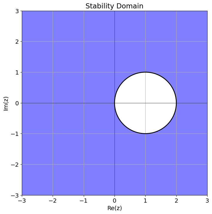
(25)#\[\begin{equation} y_{k+1} = y_{k} + \tau \lambda y_{k+1} \end{equation}\]

\[ \Leftrightarrow \; y_{k+1} = \dfrac{1}{1 - \tau \lambda} y_k = \left(\dfrac{1}{1 - \tau \lambda}\right)^{k+1} y_0. \]

Thus \(R(z) = \tfrac{1}{1-z}\). The domain of stability is \(\mathcal{S} = (-\infty, 0] \cup [2, \infty)\), in particular, no matter how we chose \(\tau\), \(|R(\lambda z)| < 1\) for \(\lambda < 0\). So the implicit Euler method is stable for the test problem ((21)), independent of the choice of the time step.

We can even plot it:

def r_fe(z):
    return 1/(1 - z)

plot_stability_domain(r_fe)

../_images/0f2c7c3bf991aa62199222af4d33455b3fdd0d940ed94eb9f5f4bd176619ae07.png

The Crank-Nicolson#

Both the explicit/forward and the implicit/backward Euler method have consistency order \(1\). Next we derive 2nd order method. We start exactly as in the derivation of Heun’s method presented in the IntroductionNuMeODE.ipynb notebook.

Again, we start from the exact integral representation, and apply the trapezoidal rule

\[\begin{align*} y(t_{k+1}) - y(t_k) &= \int_{t_k}^{t_{k+1}} f(t,y(t)) {\,\mathrm{d}t} \approx \dfrac{\tau_k}{2} \left( f(t_{k+1}, y(t_{k+1}) + f(t_{k}, y(t_{k}) \right) \end{align*}\]

This suggest to consider the implicit scheme

\[ \begin{align*} y_{k+1} &= y_k + \dfrac{\tau_k}{2} \left( f(t_{k+1}, y_{k+1}) + f(t_{k}, y_{k}) \right) \end{align*} \]

which is known as the Crank-Nicolson method.

Exercise 26 (Investigating the Crank-Nicolson method)

a) Determine the Butcher table for the Crank-Nicolson method.

Solution. We can rewrite Crank-Nicolson using two stage-derivatives \(k_1\) and \(k_2\) as follows.

\[\begin{align*} k_1 &= f(t_{k}, y_{k}) = f(t_{k} + 0 \cdot \tau, y_{k} + \tau( 0 \cdot k_1 + 0 \cdot k_2 )) \\ k_2 &= f(t_{k+1}, y_{k+1}) = f(t_{k} + 1 \cdot \tau, y_{k} + \tau(\tfrac{1}{2} k_1 + \tfrac{1}{2} k_2)) \\ y_{k+1} &= y_{k} + \tau(\tfrac{1}{2} k_1 + \tfrac{1}{2} k_2) \end{align*}\]

and thus the Butcher table is given by

\[\begin{split} \begin{array}{c|c c} 0 & 0 & 0 \\ 1 & \tfrac{1}{2} & \tfrac{1}{2} \\ \hline & \tfrac{1}{2} & \tfrac{1}{2} \end{array}. \end{split}\]

b) Use the order conditions discussed in the RungeKuttaNuMeODE.ipynb to show that Crank-Nicolson is of consistency/convergence order 2.

c) Determine the stability function \(R(z)\) associated with the Crank-Nicolson method and discuss the implications on the stability of the method for the test problem ((21)).

Solution. With \(f(t,y) = \lambda y\),

\[\begin{align*} y_{k+1} &= y_k + \dfrac{\tau}{2} \lambda y_{k+1} + \dfrac{\tau}{2} \lambda y_{k} \end{align*}\]

and thus

\[\begin{align*} y_{k+1} &= \dfrac{1+\tfrac{\tau \lambda}{2}} {1-\tfrac{\tau \lambda}{2}} y_k \end{align*}\]

and therefore

\[ R(z) = \dfrac{1+\tfrac{z}{2}} {1-\tfrac{z}{2}}. \]

As result, the stability domain \((-\infty, 0] \subset \mathcal{S}\), in particular, Crank-Nicolson is stable for our test problem, independent of the choice of the time-step.

d) Implement the Crank-Nicolson method to solve the test problem (stiff:ode:eq:exponential) numerically.

Hint. You can start from implicit_euler function implemented earlier, you only need to change a single line.

e) Check the convergence rate for your implementation by solving (stiff:ode:eq:exponential) with \(\lambda = 2\), \(t_0 = 1, T = 2\) and \(y_0 = 1\) for various time step sizes and compute the corresponding experimental order of convergence (EOC)

f) Finally, rerun the stability experiment from the section Explicit Euler method and a stiff problem with Crank-Nicolson.

Numerical solution of ordinary differential equations: Stiff problems

Contents

Numerical solution of ordinary differential equations: Stiff problems#

Explicit Euler method and a stiff problem#

The implicit Euler method#

The Crank-Nicolson#