Numerical integration: Composite quadrature rules

Numerical integration: Composite quadrature rules#

As usual, we import the necessary modules before we get started.

%matplotlib inline

import numpy as np
from numpy import pi
from math import sqrt
from numpy.linalg import solve, norm    # Solve linear systems and compute norms

import matplotlib.pyplot as plt
import matplotlib.cm as cm  

#import ipywidgets as widgets
#from ipywidgets import interact, fixed

newparams = {'figure.figsize': (16.0, 8.0), 
             'axes.grid': True,
             'lines.markersize': 8, 
             'lines.linewidth': 2,
             'font.size': 14}
plt.rcParams.update(newparams)
#plt.xkcd()

General construction of quadrature rules#

In the following, you will learn the steps on how to construct realistic algorithms for numerical integration, similar to those used in software like Matlab of SciPy. The steps are:

Construction.

Choose \(n+1\) distinct nodes on a standard interval \(I\), often chosen to be \(I=[-1,1]\).

Let \(p_n(x)\) be the polynomial interpolating some general function \(f\) in the nodes, and let the \(Q[f](-1,1)=I[p_n](-1,1)\).

Transfer the formula \(Q\) from \([-1,1]\) to some interval \([a,b]\).

Design a composite formula, by dividing the interval \([a,b]\) into subintervals and applying the quadrature formula on each subinterval.

Find an expression for the error \(E[f](a,b) = I[f](a,b)-Q[f](a,b)\).

Find an expression for an estimate of the error, and use this to create an adaptive algorithm.

Constructing quadrature rules on a single interval#

We have already seen in the previous Lecture how quadrature rules on a given interval \([a,b]\) can be constructed using polynomial interpolation.

For \(n+1\) quadrature points \(\{x_i\}_{i=0}^n \subset [a,b]\), we compute weights by

\[ w_i =\int_a^b \ell_i(x) {\,\mathrm{d}x} \quad \text{for } i = 0, \ldots, n. \]

where \(\ell_i(x)\) are the cardinal functions associated with \(\{x_i\}_{i=0}^n\) satisfying \(\ell_i(x_j) = \delta_{ij}\) for \(i,j = 0,1,\ldots, n\). The resulting quadrature rule has (at least) degree of exactness equal to \(n\).

But how to you proceed if you know want to compute an integral on a different interval, say \([c,d]\)? Do we have to reconstruct all the cardinal functions and recompute the weights?

The answer is NO! One can easily transfer quadrature points and weights from one interval to another. One typically choose the simple reference interval \(\widehat{I} = [-1, 1]\). Then you determine some \(n+1\) quadrature points \(\{\widehat{x}_i\}_{i=0}^n \subset [-1,1]\) and quadrature weights \(\{\widehat{w}_i\}_{i=0}^n\) to define a quadrature rule \(Q(\widehat{I})\)

The quadrature points can then be transferred to an arbitrary interval \([a,b]\) to define a quadrature rule \(Q(a,b)\) using the transformation

\[ x = \frac{b-a}{2}\widehat{x} + \frac{b+a}{2}, \quad \text{so} \quad {\,\mathrm{d}x} = \frac{b-a}{2}\,\mathrm{d}\widehat{x}, \]

and thus we define \(\{x_i\}_{i=0}^n\) and \(\{w_i\}_{i=0}^n\) by

\[ x_i = \frac{b-a}{2}\widehat{x}_i + \frac{b+a}{2}, \quad w_i = \frac{b-a}{2}\widehat{w}_i \quad \text{for } i = 0, \ldots n. \]

Example: Simpson’s rule

Choose standard interval \([-1,1]\). For Simpson’s rule, choose the nodes \(x_0=-1\), \(x_1=0\) and \(x_2=1\). The corresponding cardinal functions are
- \(\displaystyle \ell_0 = \frac{1}{2}(x^2-x), \qquad \ell_1(x) = 1-x^2, \qquad \ell_2(x) = \frac{1}{2}(x^2+x). \)

which gives the weights

\(\displaystyle w_0 = \int_{-1}^1 \ell_0(x)dx = \frac{1}{3}, \qquad w_1 = \int_{-1}^1 \ell_1(x)dx = \frac{4}{3}, \qquad w_2 = \int_{-1}^1 \ell_2(x)dx = \frac{1}{3}\)

such that

\( \displaystyle \int_{-1}^1 f(t) dx \approx \int_{-1}^1 p_2(x) dx = \sum_{i=0}^2 w_i f(x_i) = \frac{1}{3} \left[\; f(-1) + 4 f(0) + f(1) \; \right].\)

After transferring the nodes and weights, Simpson’s rule over the interval \([a,b]\) becomes
- \(\displaystyle S(a,b) = \frac{b-a}{6}\left[\; f(a)+4f(c)+f(b)\; \right], \qquad c=\frac{b+a}{2}\).

Composite quadrature rules#

To generate more accurate quadrature rule \(Q(a,b)\) we have in principle two possibilities:

Increase the order of the interpolation polynomial used to construct the quadrature rule.

Subdivide the interval \([a,b]\) into smaller subintervals and apply a quadrature rule on each of the subintervals, leading to Composite Quadrature Rules which we will consider next.

colors = plt.get_cmap("Pastel1").colors

def plot_cqr_examples(m):
    f = lambda x : np.exp(x)
    fig, axs = plt.subplots(1,2)
    fig.set_figheight(4)
    fig.set_figwidth(fig.get_size_inches()[0]*1)
    #axs[0].add_axes([0.1, 0.2, 0.8, 0.7])
    a, b = -0.5,0.5
    l, r = -1.0, 1.0
    x_a = np.linspace(a, b, 100)
    

    for ax in axs:
        ax.set_xlim(l, r)
        x = np.linspace(l, r, 100)
        ax.plot(x, f(x), "k--", label="$f(x)$")
        #ax.fill_between(x_a, f(x_a), alpha=0.1, color='k')
        ax.xaxis.set_ticks_position('bottom')
        ax.set_xticks([a,b])
        ax.set_xticklabels(["$a$", "$b$"])
        ax.set_yticks([])
        ax.legend(loc="upper center")
    
    h = (b-a)/m
    # Compute center points for each interval
    xcs = np.linspace(a+h/2, b-h/2, m)
    xis = np.linspace(a,b,m+1)
    

    # Midpoint rule
    axs[0].bar(xis[:-1], f(xcs), h, align='edge', color=colors[2], edgecolor="black")
    axs[0].plot(xcs,f(xcs), 'ko', markersize=f"{6*(m+1)/m}")
    axs[0].set_title("Composite midpoint rule")


    # Trapezoidal rule
    axs[1].set_title("Composite trapezoidal rule")
    axs[1].fill_between(xis, f(xis), alpha=0.8, color=colors[4])
    axs[1].plot(xis,f(xis), 'ko', markersize=f"{6*(m+1)/m}")
    plt.vlines(xis, 0, f(xis), colors="k")
    plt.show()

import ipywidgets as widgets
from ipywidgets import interact

slider = widgets.IntSlider(min = 1,
                           max = 20,
                           step = 1,
                           description="Number of subintervals m",
                           value = 1)
interact(plot_cqr_examples, m=slider)

<function __main__.plot_cqr_examples(m)>

m = 4
plot_cqr_examples(m)

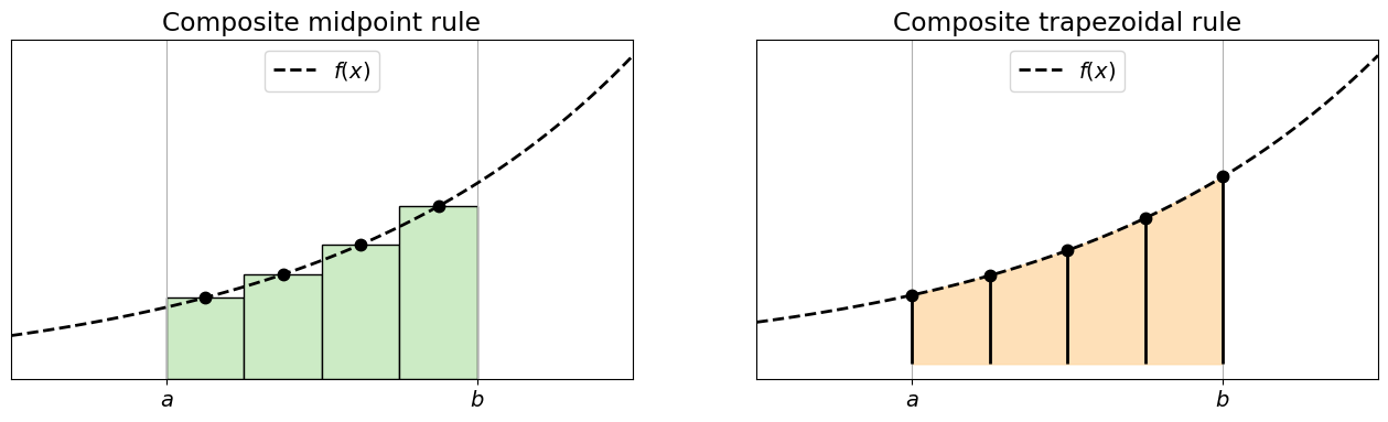
../_images/338afbf6de700019c123d938342f13c328daa95f3a8b5fd047e18ff710566d5c.png

Select \(m \geqslant 1\) and divide \([a,b]\) into \(m\) equally spaced subintervals \([x_{i-1}, x_{i}]\) defined by \(x_i = a + i h\) with \(h = (b-a)/m\) for \(i=1,\ldots, m\). Then for a given quadrature rule \(\mathrm{Q}[\cdot](x_{i-1},x_i)\) the corresponding composite quadrature rule \(\mathrm{CQ}[\cdot]({[x_{i-1}, x_{i}]}_{i=1}^{m})\) is given by

\[ \int_a^b f {\,\mathrm{d}x} \approx \mathrm{CQ}[f]({[x_{i-1}, x_{i}]}_{i=1}^{m}) = \sum_{i=1}^m \mathrm{Q}[f](x_{i-1},x_i). \]

(eqquad:composite_qr}

Composite trapezoidal rule#

Using the trapezoidal rule

\[ \mathrm{T}[f](x_{i-1},x_{i}) = \tfrac{h}{2} f(x_{i-1}) + \tfrac{h}{2} f(x_{i}) \]

the resulting composite trapezoidal rule is given by

\[\begin{align*} \int_a^b f {\,\mathrm{d}x} \approx \mathrm{CT}[f]({[x_{i-1}, x_{i}]}_{i=1}^{m}) = h \left[ \tfrac{1}{2} f(x_0) + f(x_1) + \ldots + f(x_{m-1}) + \tfrac{1}{2} f(x_m) \right] \end{align*}\]

Exercise 9 (Testing the accuracy of the composite trapezoidal rule)

Have a look at the CT function which implements the composite trapezoidal rule:

def CT(f, a, b, m):
    """ Computes an approximation of the integral f
    using the composite trapezoidal rule.
    Input:
        f:  integrand
        a:  left interval endpoint
        b:  right interval endpoint
        m:  number of subintervals
    """
    x = np.linspace(a,b,m+1)
    h = float(b - a)/m
    fx = f(x[1:-1])
    ct = h*(np.sum(fx) + 0.5*(f(x[0]) + f(x[-1])))
    return ct

Use this function to compute an approximate value of integral

\[ I(0,1) = \int_0^1 \cos\left(\frac{\pi}{2}x\right) = \frac{2}{\pi} = 0.636619\dotsc. \]

for \(m = 4, 8, 16, 32, 64\) corresponding to \( h = 2^{-2}, 2^{-3}, 2^{-4}, 2^{-5}, 2^{-6}\). Tabulate the corresponding quadrature errors \(I(0,1) - Q(0,1)\). What do you observe?

# Insert your code here

def f(x):
    return np.cos(np.pi/2*x)

a, b = 0, 1
m = 2
int_f = 2/np.pi

qr_f = CT(f, a, b, m)
print(f"Exact value {int_f}")
print(f"Numerical integration for m = {m} gives {qr_f}")
print(f"Difference  = {int_f - qr_f}")

for m in [4, 8, 16, 32, 64]:
    qr_f = CT(f, a, b, m)
    print(f"Exact value {int_f}")
    print(f"Numerical integration for m = {m} gives {qr_f}")
    print(f"Difference  = {int_f - qr_f}")

Exact value 0.6366197723675814
Numerical integration for m = 2 gives 0.6035533905932737
Difference  = 0.03306638177430765
Exact value 0.6366197723675814
Numerical integration for m = 4 gives 0.6284174365157311
Difference  = 0.008202335851850262
Exact value 0.6366197723675814
Numerical integration for m = 8 gives 0.6345731492255537
Difference  = 0.002046623142027637
Exact value 0.6366197723675814
Numerical integration for m = 16 gives 0.6361083632808496
Difference  = 0.0005114090867317511
Exact value 0.6366197723675814
Numerical integration for m = 32 gives 0.6364919355013015
Difference  = 0.00012783686627992896
Exact value 0.6366197723675814
Numerical integration for m = 64 gives 0.636587814113642
Difference  = 3.195825393942364e-05

Solution to Exercise 9 (Testing the accuracy of the composite trapezoidal rule)

# Define function
def f(x):
    return np.cos(pi*x/2)

# Exact integral
int_f = 2/pi 

# Interval
a, b = 0, 1

# Compute integral numerically
for m in [4, 8, 16, 32, 64]:
    cqr_f = CT(f, a, b, m)
    print(f"I[f] = {int_f}")
    print(f"Q[f, {a}, {b}, {m}] = {qr_f}")
    print(f"I[f] - Q[f] = {int_f - qr_f:.3e}")

Remark 3

We observe that for each doubling of the number of subintervals we decrease the error by a fourth. That means that if we look at the quadrature error \(I[f]-\mathrm{CT}[f]\) as a function of the number of subintervals \(m\) (or equivalently as a function of \(h\)), then \(|I[f]-\mathrm{CT}[f]| \approx \tfrac{C}{m^2} = C h^2\).

Error estimate for the composite trapezoidal rule#

We will now theoretically explain the experimentally observed convergence rate in the previous Exercise 9.

First we have to recall the error estimate for for the trapezoidal rule on a single interval \([a,b]\). If \(f\in C^2(a,b)\), then there is a \(\xi \in (a,b)\) such that

\[ I[f]-\mathrm{T}[f]=\frac{(b-a)^3}{12}f''(\xi). \]

Theorem 7 (Quadrature error estimate for composite trapezoidal rule)

Let \(f\in C^2(a,b)\), then the quadrature error \(I[f]-\mathrm{CT}[f]\) for the composite trapezoidal rule can be estimated by

(4)#\[\begin{equation} |I[f]-\mathrm{CT}[f]| \leqslant \dfrac{M_2}{12} \dfrac{(b-a)^3}{m^2} = \dfrac{M_2}{12} h^2(b-a) \end{equation}\]

where \(M_2 = \max_{\xi\in[a,b]} |f''(\xi)|\).

Proof.

\[\begin{align*} |I[f]-\mathrm{CT}[f]| &= \biggl \lvert \sum_{i=1}^m \Bigl [ \int_{x_{i-1}}^{x_i} f(x) {\,\mathrm{d}x} - \bigl( \tfrac{h}{2}f(x_{i-1}) + \tfrac{h}{2}f(x_{i}) \bigr) \Bigr] \biggr \rvert \\ &\leqslant \sum_{i=1}^m \frac{h^3}{12}|f''(\xi_i)| \leqslant M_2 \sum_{i=1}^m \frac{(h)^3}{12} \leqslant M_2 \sum_{i=1}^m \frac{(h)^3}{12} \\ &= M_2 \frac{h^3}{12} \underbrace{m}_{\tfrac{(b-a)}{h}} = \dfrac{M_2}{12} h^2(b-a) = \frac{M_2}{12} \frac{(b-a)^3}{m^2} \end{align*}\]

Interlude: Convergence of \(h\)-dependent approximations#

Let \(X\) be the exact solution, and \(X(h)\) some numerical solution depending on a parameter \(h\), and let \(e(h)\) be the norm of the error, so \(e(h)=\|X-X(h)\|\). The numerical approximation \(X(h)\) converges to \(X\) if \(e(h) \rightarrow 0\) as \(h\rightarrow 0\). The order of the approximation is \(p\) if there exists a positive constant \(M\) such that

\[ e(h) \leq M h^p \]

This is often expresed using the Big \(\mathcal{O}\)-notation,

\[ e(h) = \mathcal{O}(h^p) \qquad\text{ as } h \to 0. \]

This is often used when we are not directly interested in any expression for the constant \(M\), we only need to know it exists.

Again, we see that a higher approximation order \(p\) leads for small values of \(h\) to a better approximation of the solution. Thus we are generally interested in approximations of higher order.

Numerical verification

The following is based on the assumption that \(e(h)\approx C h^p\) for some unknown constant \(C\). This assumption is often reasonable for sufficiently small \(h\).

Choose a test problem for which the exact solution is known and compute the error for a decreasing sequence of \(h_k\)’s, for instance \(h_k=H/2^k\), \(k=0,1,2,\dots\). The procedure is then quite similar to what was done for iterative processes.

\[\begin{split} \begin{array}{rcl} e(h_{k+1}) &\approx& C h_{k+1}^p \\ e(h_k) &\approx& C h_k^p \end{array} \qquad \Rightarrow \qquad \frac{e(h_{k+1})}{e(h_k)} \approx \left( \frac{h_{k+1}}{h_k} \right)^p \qquad \Rightarrow \qquad p \approx \frac{\log{(e(h_{k+1})/e(h_k))}}{\log{(h_{k+1}/h_k)}} \end{split}\]

For one refinement step where one passes from \(h_k \to h_{k+1}\), the number

\[ EOC(k) \approx \frac{\log{(e(h_{k+1})/e(h_k))}}{\log{(h_{k+1}/h_k)}} \]

is often called the “Experimental order of convergence at refinement level k”

Since

\[ e(h) \approx Ch^p \qquad \Rightarrow \qquad \underbrace{\log{e(h)}}_{y} \approx \underbrace{\log{C}}_{a} + p \underbrace{\log{h}}_{x} \]

a plot of \(e(h)\) as a function of \(h\) using a logarithmic scale on both axes (a log-log plot) will be a straight line with slope \(p\). Such a plot is referred to as an error plot or a convergence plot.

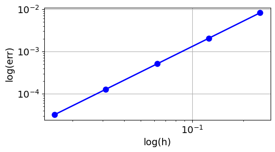
Exercise 10 (Convergence order of composite trapezoidal rule)

Examine the convergence order of composite trapezoidal rule.

# Insert your code here.

Solution to Exercise 10 (Convergence order of composite trapezoidal rule)

# Define function
def f(x):
    return np.cos(pi*x/2)

# Exact integral
int_f = 2/pi 

# Interval
a, b = 0, 1

errs = []
hs = []

# Compute integral numerically
for m in [4, 8, 16, 32, 64]:
    cqr_f = CT(f, a, b, m)
    print("Number of subintervals m = {}".format(m))
    print("Q[f] = {}".format(cqr_f))
    err = int_f - cqr_f
    errs.append(err)
    hs.append((b-a)/m)
    print("I[f] - Q[f] = {:.10e}".format(err))

hs = np.array(hs)
errs = np.array(errs)

eocs = np.log(errs[1:]/errs[:-1])/np.log(hs[1:]/hs[:-1])
print(eocs)
plt.figure(figsize=(6, 3)) 
plt.loglog(hs, errs, "bo-")
plt.xlabel("log(h)")
plt.ylabel("log(err)")

# Adding infinity in first row to eoc list
# to make it the same length as errs
eocs = np.insert(eocs, 0, np.inf)

Number of subintervals m = 4
Q[f] = 0.6284174365157311
I[f] - Q[f] = 8.2023358519e-03
Number of subintervals m = 8
Q[f] = 0.6345731492255537
I[f] - Q[f] = 2.0466231420e-03
Number of subintervals m = 16
Q[f] = 0.6361083632808496
I[f] - Q[f] = 5.1140908673e-04
Number of subintervals m = 32
Q[f] = 0.6364919355013015
I[f] - Q[f] = 1.2783686628e-04
Number of subintervals m = 64
Q[f] = 0.636587814113642
I[f] - Q[f] = 3.1958253939e-05
[2.00278934 2.00069577 2.00017385 2.00004346]

../_images/42325cce18e4d79699df5893434193e8ffde2b1841ce592e9af2b5dcf28add70.png

# Do a pretty print of the tables using panda
import pandas as pd
#from IPython.display import display

table = pd.DataFrame({'Error': errs, 'EOC' : eocs})
display(table)
print(table)

	Error	EOC
0	0.008202	inf
1	0.002047	2.002789
2	0.000511	2.000696
3	0.000128	2.000174
4	0.000032	2.000043

      Error       EOC
0.008202       inf
0.002047  2.002789
0.000511  2.000696
0.000128  2.000174
0.000032  2.000043

Exercise 11 (Composite Simpson’s rule)

The composite Simpson’s rule is considered in detail in homework assignment 2.

Theorem 8 (Quadrature error estimate for composite Simpon’s rule)

Let \(f\in C^4(a,b)\), then the quadrature error \(I[f]-\mathrm{CT}[f]\) for the composite trapezoidal rule can be estimated by

(5)#\[\begin{equation} |I[f]-\mathrm{CSR}[f]| \leqslant \dfrac{M_4}{2880} \dfrac{(b-a)^5}{m^4} = \dfrac{M_4}{2880} h^4(b-a) \label{quad:thm:csr_est} \tag{3} \end{equation}\]

where \(M_4 = \max_{\xi\in[a,b]} |f^{(4)}(\xi)|\).

Proof.

Will be part of homework assignment 2.